How to Highlight Duplicates in Google Sheets? [2025]

Are you seeing double, or is your spreadsheet playing tricks on you? We've all been there: scrolling through multiple rows and multiple columns of data, trying to spot patterns and aggregate figures. Then it hits you. Some of this info looks familiar. Those are duplicates and can mar the value you get from data.
In this article, you'll learn how to highlight duplicates in Google Sheets using different methods.
Step-by-Step Guide on How to Highlight Duplicates in Google Sheets
You can highlight duplicates in Google Sheets using the conditional formatting rule. Below, you'll get access to step-by-step instructions for using this feature and screenshots or images to guide the reader through the process visually.
Highlighting Duplicates in a Single Column — Column-specific formatting
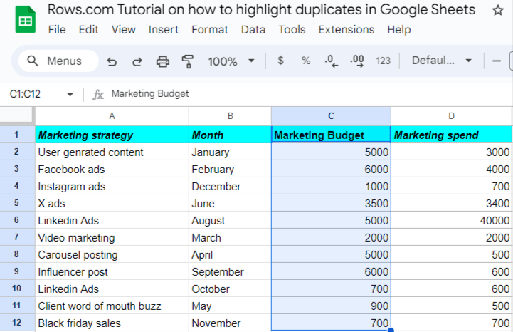
Step 1: Highlight the specific column you want to check for duplicates.
Select the range you want to check (C1:C12) in this case).
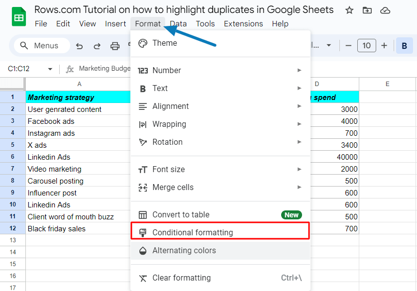
Step 2: Click “format” in the top menu. Afterward, you'll see a pop-up of various format functions; click “Conditional formatting.”
After step 2, you'll see a box on the right-hand side of your screen showing — the conditional format rule. This editing box helps you carry out the format rules, and edit color style for highlighting.
Step 3: Click “format rules” and choose “custom formula is.” You'll have to scroll down a bit to see it.
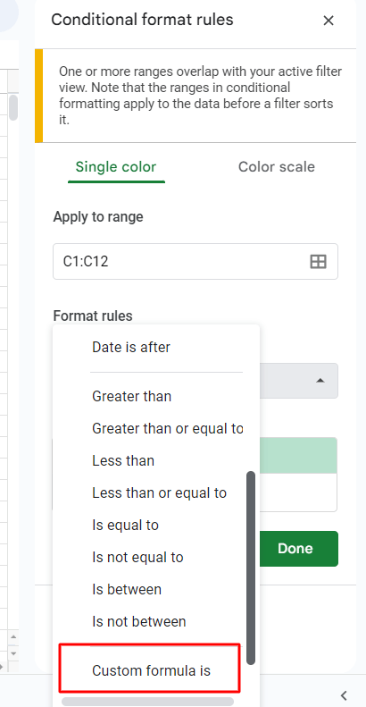
Step 4: Use the COUNTIF formula and add specific parameters related to your highlighted column.
If you want to find out how many times each value appears in a range, you can use:
=COUNTIF(A:A, A1) >1
This formula counts how many times the same value used in cell A1 appears in the entire column A.
If the result is greater than 1, the first value is duplicated.
Or you use : =COUNTIF ($X$X, $X, X1)>1]
Where,
X is the alphabet of your column.
For this example, we are trying to check for duplicates in the C column, so we used this formula:
The dollar sign ($) in formulas creates absolute references. An absolute reference means that when you copy the formula to another cell, the reference to the cell with the dollar sign will not change.
The COUNTIF formula tells Sheets where to look for duplicates.
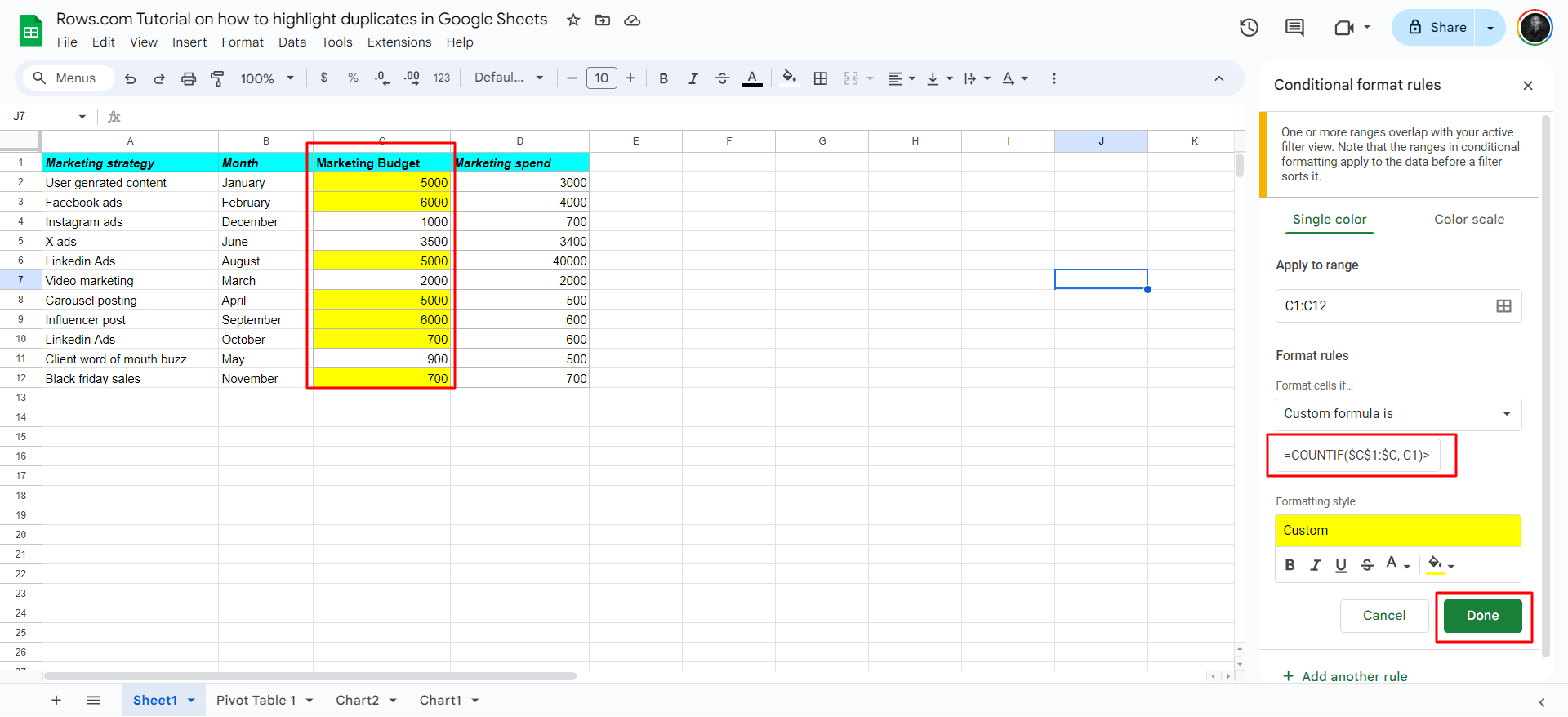
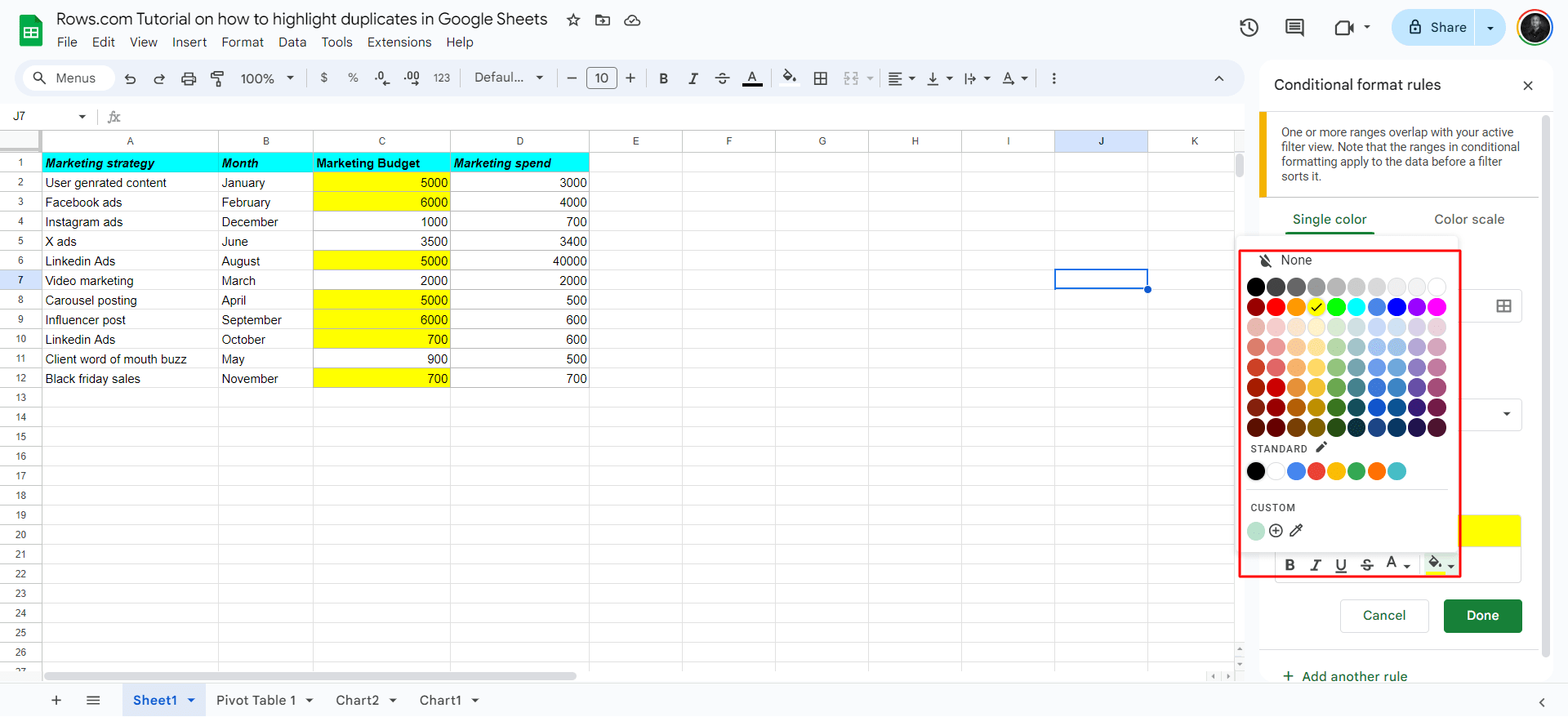
After inserting your formula, you may notice highlighted cells in your Sheets, showing that your work is done. But to add some finesse, you can edit the color style of the highlighted portions.

The spreadsheet for modern teams
Save hours on data import, surface insights by asking, and share beautiful, ready-to-use dashboards.
Get Started (free)Highlighting Duplicates Across Multiple Columns
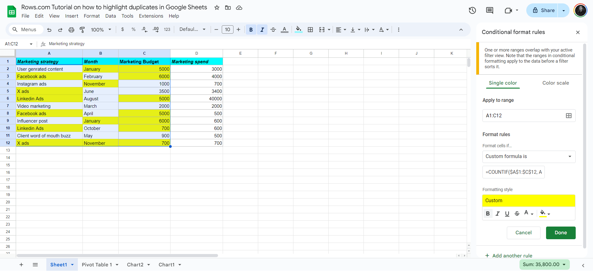
Duplicates can exist in various columns in your Sheets. To highlight cross-column duplicates, follow the steps below —
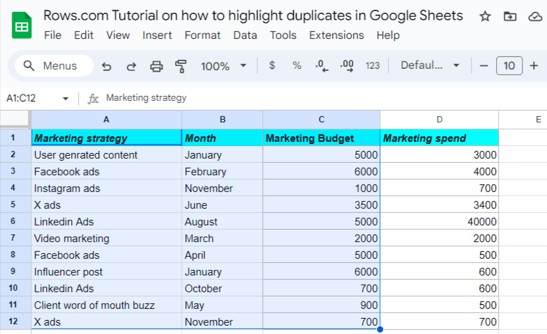
Step 1: Select the range you want to check (A1:D12).
For this example, we highlight columns A, B, and C.
Use this formula —
=COUNTIF($A$1:$C$12, A1) > 1
When inputting the formula, choose from the beginning of the range to the end of the range. This means if you choose columns A, B, and C, start from A1 to the last cells of the C column.
Follow steps 2 and 3 in the section above to highlight a single column.
Afterwards, insert the formula. Click “Done” to see the highlighted duplicates.
How to highlight duplicates using the UNIQUE function
The UNIQUE function itself doesn't directly highlight duplicates in multiple fashion like the conditional format rule. Its primary purpose is to return a list of unique values from a range. However, we can use it as a strategy to identify duplicates.
In a separate column (let's say column D), use this formula:
=UNIQUE (RANGE)
=UNIQUE (C2:C12)
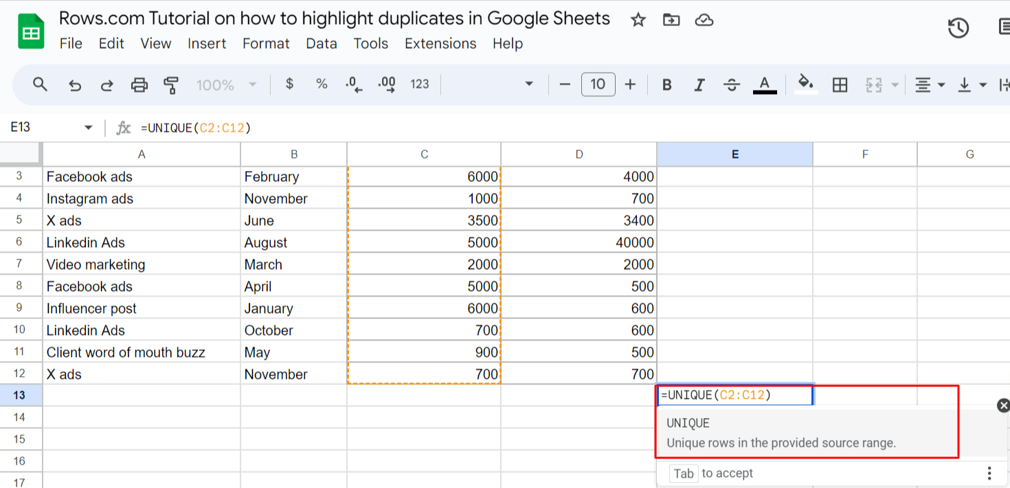
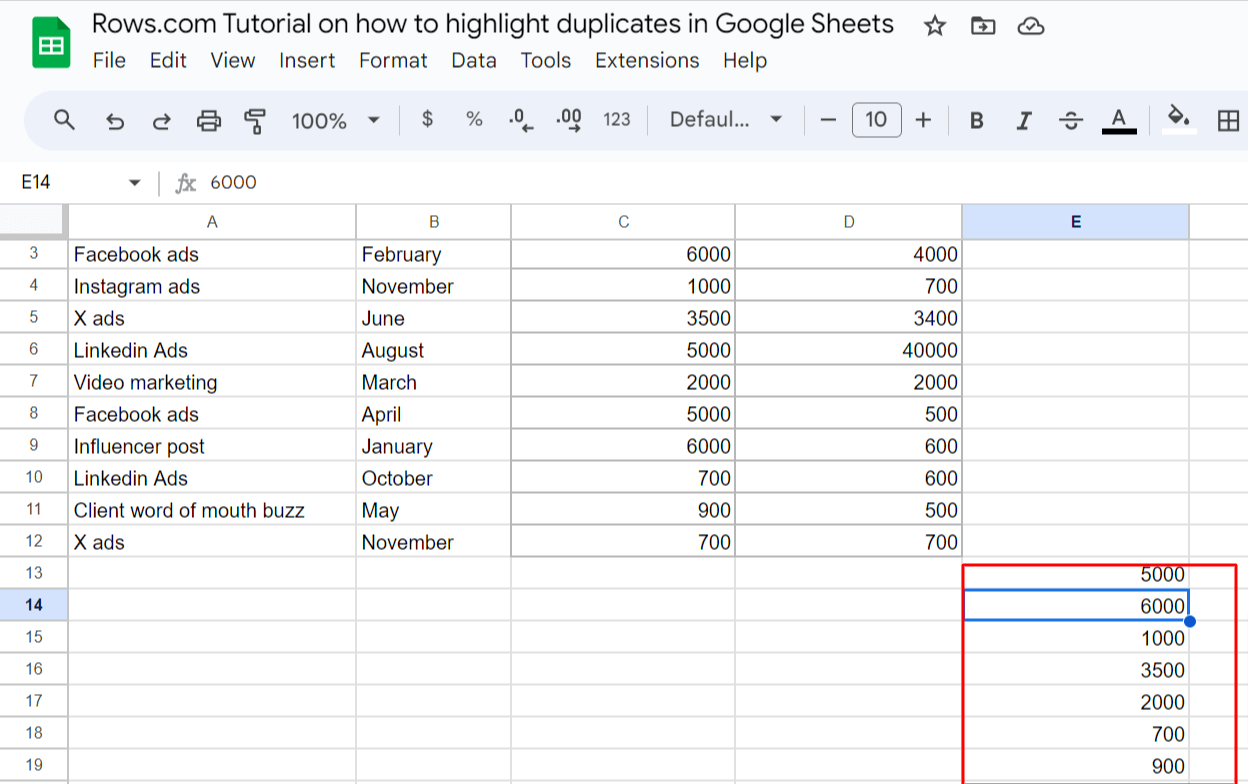
Once inserted, click the “enter” tab on your keyboard, and you'll get a list of characters that appeared twice or more in your sheets.
How to Remove Duplicates After Highlighting Them
You can remove duplicates in Google Sheets by using the data cleanup feature. By using the data cleanup feature, you are maintaining an accurate and efficient spreadsheet.
Here's a step-by-step guide on removing duplicates after highlighting them, ensuring your data remains clean and optimized.
Step 1. Backup Your Data
Before making any changes:
Create a copy of your spreadsheet
This safeguards your information in case of accidental deletions.
Step 2. Highlight Duplicates
Use built-in tools to identify duplicates:
In Google Sheets: Data > Conditional Formatting > Highlight duplicates — Use the steps above to highlight them and review highlighted Entries. Manually scan the highlighted cells to ensure you're comfortable removing them.
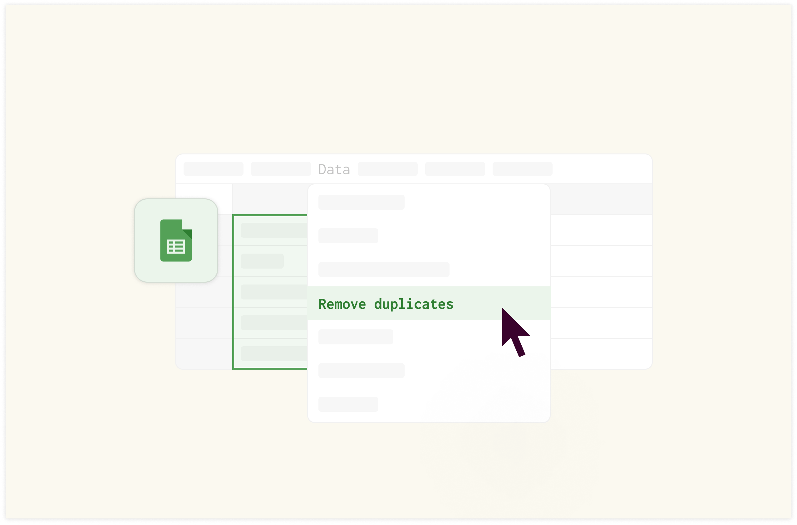
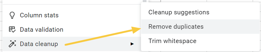
Step 3: Click on the column where you want to delete duplicates. Then click “Data.” Once done, you'll get various “Data” functions. Click ”Data cleanup” and you'll see a popup of three other sub-functions — Choose “Remove duplicates.”
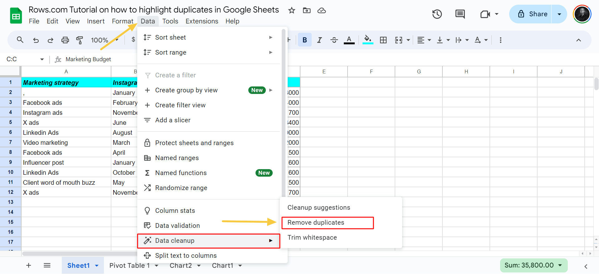
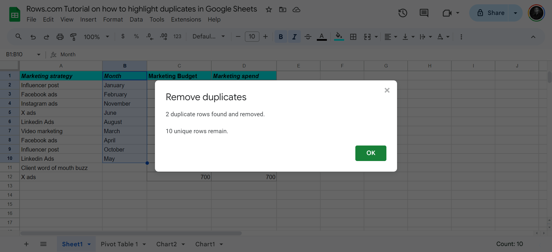
Step 4: Click “ok,” and you'll find that the duplicates for that specific column are gone.
ICYMI: Best 15 Free Google Sheets Dashboard Templates [2025].
Common Mistakes to Avoid When Finding Duplicates in Google Sheets
It is easy to make errors that compromise your results when finding duplicates. Here are the most common mistakes and how to avoid them:
Ignoring Partial Matches
Entries like "John Doe" and "John" might be duplicates in your context but won't be caught by basic duplicate checks.
Fix: Find partial matches using the SEARCH() function in your conditional formatting.
Not Updating Rules for New Data
As you add new rows or columns, your conditional formatting rules and formatting style might not automatically extend to cover them.
How to fix: Regularly review and update your formatting rules. Use absolute reference to range (e.g., $A$1:$A) to ensure rules apply to entire columns.
Ignoring Case Sensitivity
Many users forget that Google Sheets treats "Data" and "data" as different entries by default.
How to fix: When setting up multiple conditional formatting rules, choose "Custom formula is" and use the LOWER() function to convert all text to lowercase before comparing:
=COUNTIF(LOWER($A$1:$A), LOWER(A1))>1
How do these mistakes lead to failure? Well, check this out —
A marketing team relied on a spreadsheet to track customer interactions. Due to case-sensitive duplicate detection, they failed to notice multiple entries for the same client, leading to redundant outreach and damaged client relationships.
By avoiding these common mistakes, you'll improve the accuracy of your duplicate detection in Google Sheets. Remember, regular audits of your data entrt and formatting rules are key to maintaining data integrity.
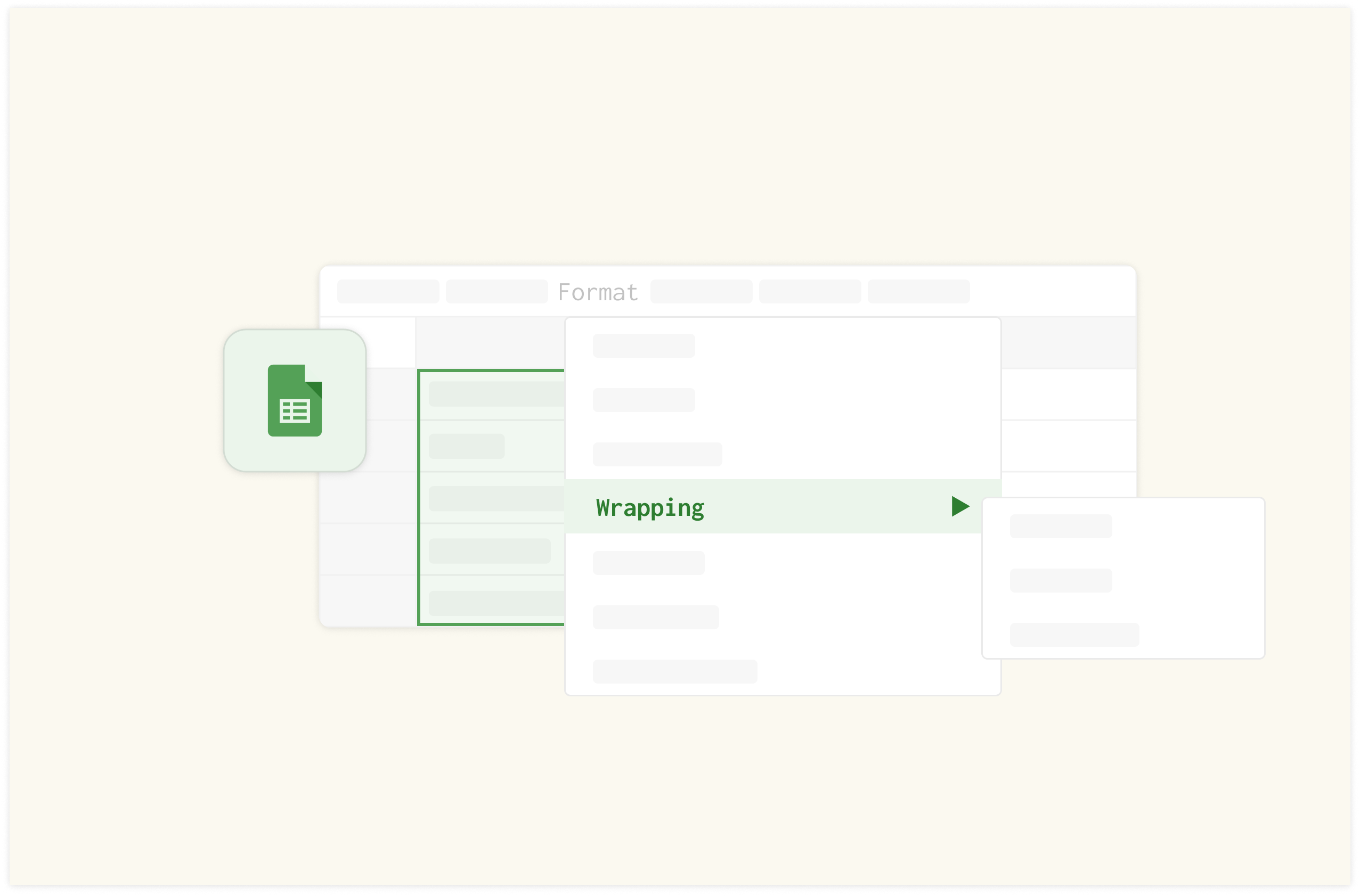
Recent reads: How to Wrap Text in Google Sheets [2025].
How to highlight duplicates in Rows

Rows is a comprehensive spreadsheet for modern teams that offers a better interface, built-in integrations for data ingestion and has native AI capabilities (AI analyst, AI-generated subtitles, native AI functions).
To find duplicates in Rows, follow the three methods below — the first of the three methods is very unique when compared to finding duplicates in Google Sheets.
Method #1 — Using EXTRACT OPENAI extract function
With the EXTRACT_OPENAI function in Rows, you can easily find duplicates in your spreadsheet.
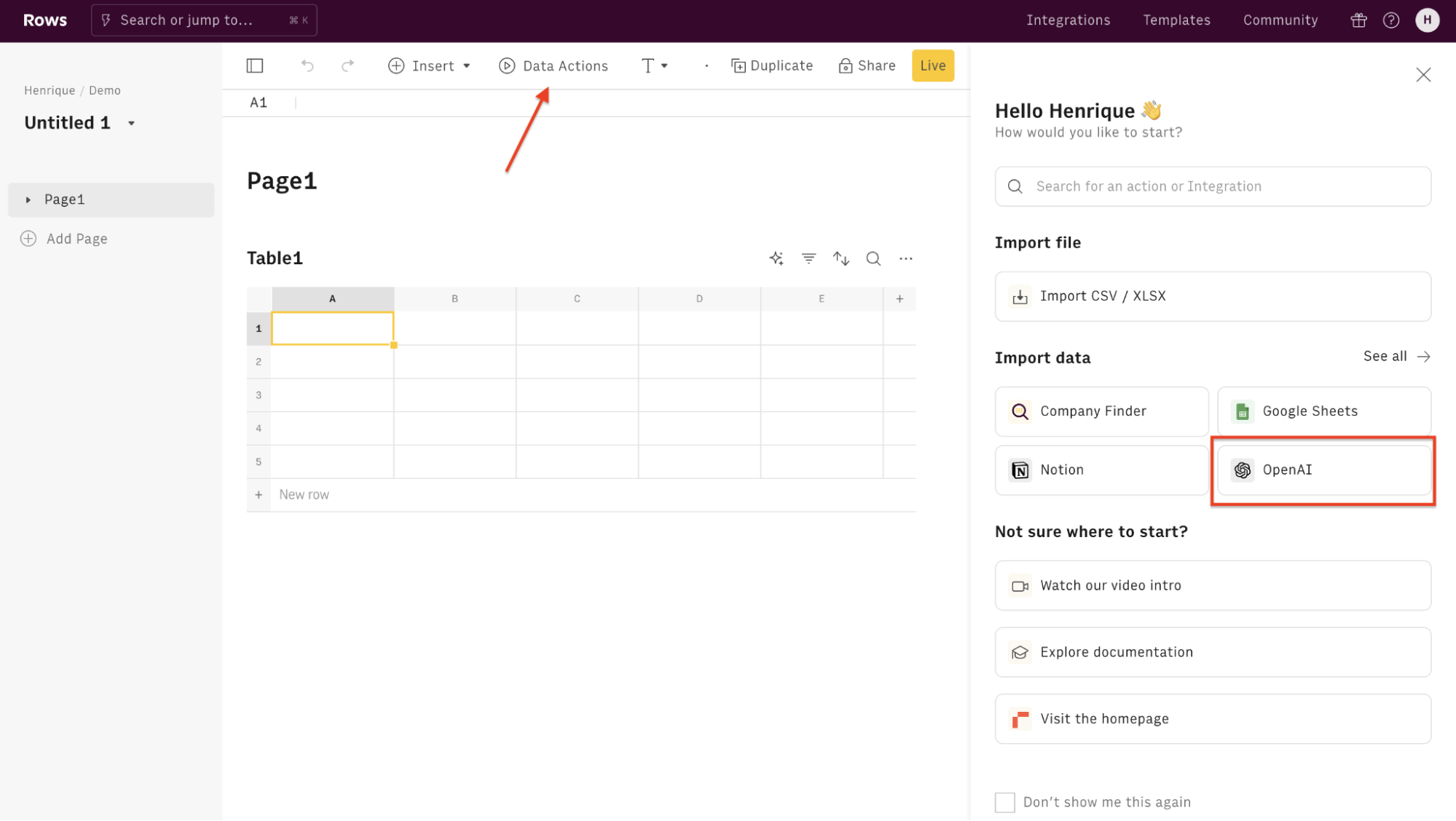
To use this function you need to connect OpenAI to Rows: open a new spreadsheet, and select the OpenAI on the welcome side panel. Alternatively, you can search for the integration inside the Data actions panel.
Inside the Data Actions panel, search for "Extract" and select one of the following actions.
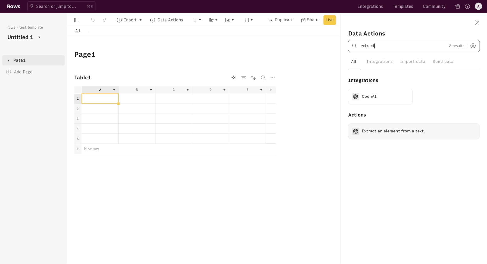
Finally, Connect the integration to get started.
The Free plan includes 20 free uses of the OpenAI integration. Users on the Plus or Pro plans have unlimited access to OpenAI and can use their API key to access any OpenAI model, including fine-tuned models. By default, the OpenAI integrations use the latest "gpt-4o" model.
After integrating your GPT account to Rows, proceed to extracting the duplicate characters in your data sheet.
Use these syntax;
=EXTRACT_OPENAI (“only duplicate values”, data range)
For this example, we are checking duplicates in the first column of the sheet.
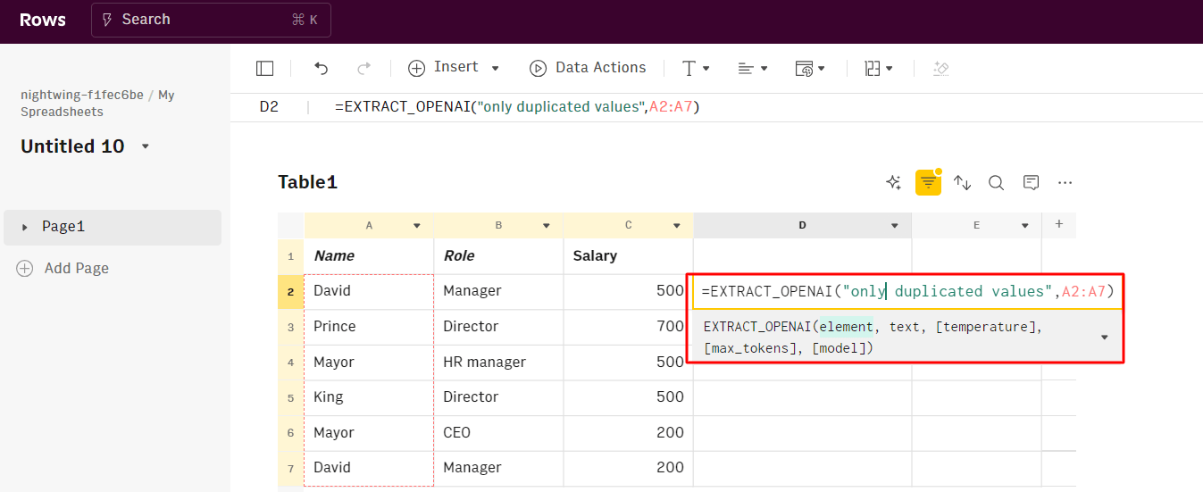
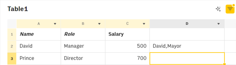
Once inputted, press the “enter tab on your keyboard. And you'll get the extracted characters that appear more than once in a specific column.
Method #2 — Using COUNTIF function
Rows has the COUNTIF and conditional formatting rule, but there's no custom formula in conditional formatting — this means you can execute formatting style edit.
That means — you need to create a support column and apply the formatting there.
In Rows, you can refer to unbounded ranges (e.g. A:A) without dollarizing the syntax — e.g. $A$2:$A$1. This is very convenient when new cells are populated in column A.
To use COUNTIF on Rows, follow these steps:
Type in the syntax with the range you want to check. Note — In Rows, you only specify a column because the custom formula is lacking.
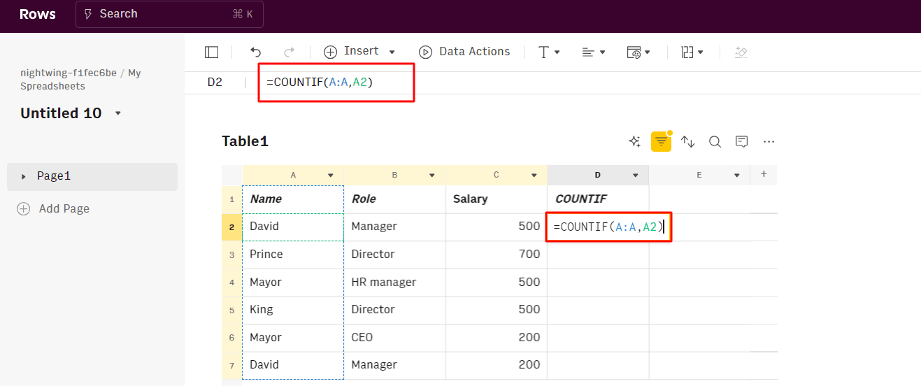
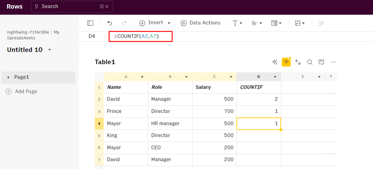
Press enter and do same execution for other cell references to find out if they are duplicates.
Method #3 — Using UNIQUE function
When compared to executing UNIQUE syntax in Google Sheets — Rows stands out because it creates a separate table of unique values and strings, resulting in a tidier, more organized output.
Below are step by step instructions on how to use the UNIQUE function to draft duplicate data entries in your data spreadsheet:
Type in the UNIQUE syntax in a separate cell.
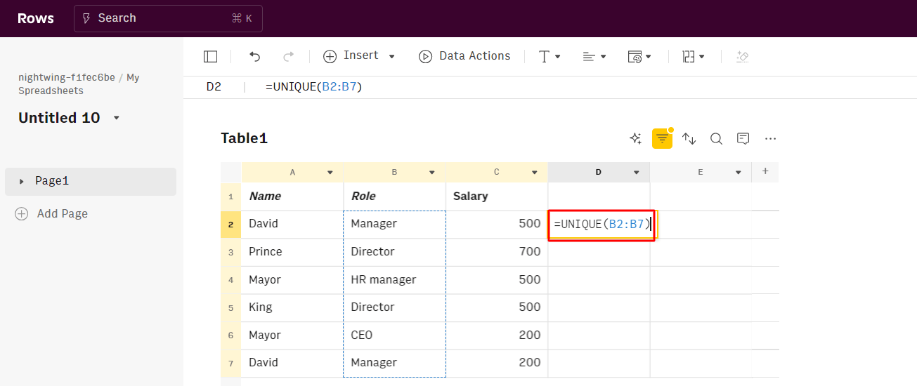
For this example, we are trying to draft out duplicate character in B column.
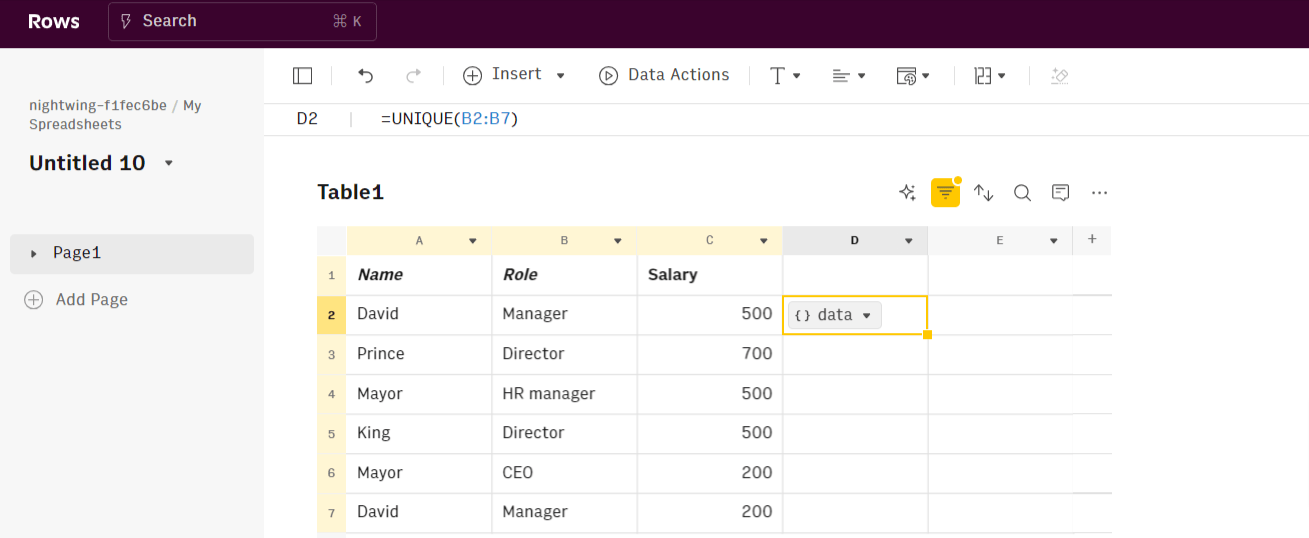
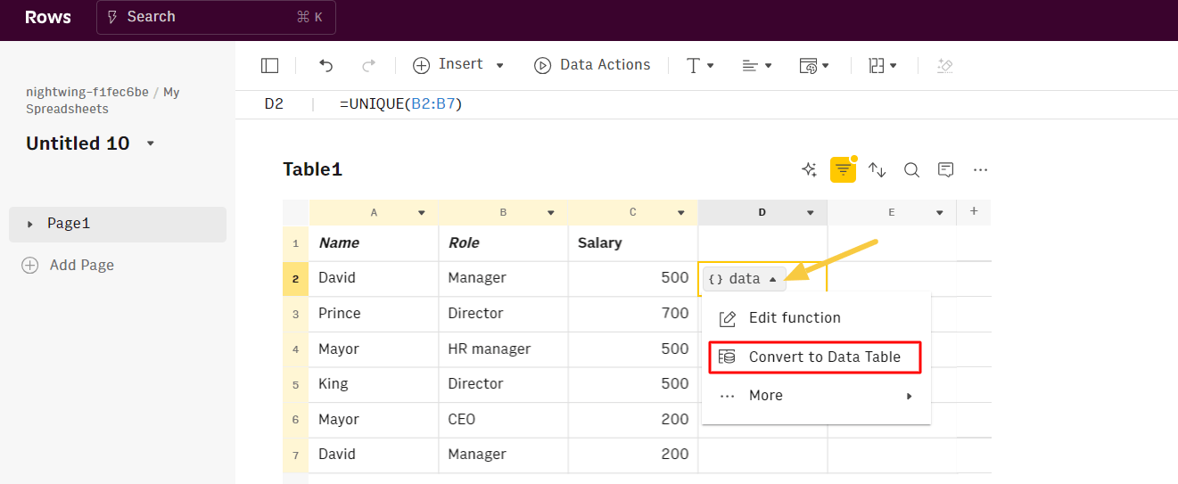
Once inserted. You'll see a data tab with a drop down arrow — click it.
Once done, you'll get a menu of different functions. Click “Convert to Data table” — this function create a separate table to show you characters that appeared more than once.
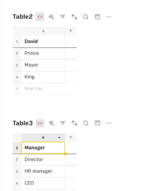
Here are a few clicks of the results for both A and B cells —
Related: How to Create and use Pivot Tables in Google Sheets [2025].
The spreadsheet for modern teams
Save hours on data import, surface insights by asking, and share beautiful, ready-to-use dashboards.
Get Started (free)Rows top features compared to Google Sheets
Below are some Row tops features that makes it unique for drafting duplicates and for general spreadsheet purposes —
Data aggregation — OpenAI integration
You can aggregate live data from 50+ sources in a very simple manner, thanks to built-in data integrations in various domains:
Marketing: GA4, GSC, Facebook, Instagram, TikTok, etc
Productivity software: OpenAI, Notion, Slack, Email, Translate
Data Warehouse: MySQL, BigQuery, PostgreSQL, Snowflake, Amazon Redshift
And many more.
The main emphasis of the data feature is the OpenAI integration.
With the OPENAI feature integration and EXTRACT_OPENAI function, you can carry out extractions of vital characters or insights in your spreadsheet —
There are several ways to use OpenAI for data extraction:
Extract feature requests from users' feedback: Discover your customers' expectations by extracting what they would love to see in your product.
Extract contact details from emails: Extract email address or phone number from your clients' email replies.
Extract a portion of unformatted JSON: Clean up a JSON by extracting all chars before or after a specific delimiter.
Extract key insights from surveys: Go straight to the point and analyze the response to open-ended questions.
Extract details from full addresses: Clean up a list of addresses extracting Zip codes and cities.
AI-powered automation
With the AI Analyst, you can ask AI to analyze, summarize, transform, and enrich your analysis. Click on the "AI Analyst“ ✨ icon, at the top right corner of any table.
A chat interface will open on the right: you can ask a broad range of questions, from basic spreadsheet commands - plotting a chart or adding or formatting columns - to more complex tasks, such as slicing, pivoting, or computing metrics about your data.
For example, given a dataset with daily revenue and costs of various marketing campaigns, you can ask the Analyst to add a column with the profit margin. Watch the video below:
In addition, our AI Analyst is instructed to use our native OpenAI functions to perform data enrichment or extraction tasks.
For example, you can ask the AI analyst to run a sentiment analysis on a column with product reviews, or add a column that categorizes addresses into regions, see below:
Want to know more about how our Analyst works? Check out our guide or watch our demo.
Modern UI
Spreadsheets in Rows present a document-like layout with standalone tables and charts that are stacked vertically and horizontally.
WYSIWYG: the spreadsheet IS the dashboard. All data is rendered as regular spreadsheet tables. And you can move elements vertically and horizontally with drag&drop. And if something breaks, you can intervene on that table or chart very flexibly, without the need to dive into complex workflows.
View Mode: View mode makes your spreadsheets work like web applications. With input fields, you can help anyone understand how to use your spreadsheet by highlighting the cells that need an input by the user.
Supercharge your sheets with Rows
With Rows, you get access to 50+ built-in data source integrations in various domains.
This makes it easy to ingest data into your table quickly and reduces your team's stress. With Rows, you can gather data from various sources in your system. This allows for more detailed analyses and helps your team uncover insights they might miss.
Ready to get started with Rows.com? Start using the product right away for free.