How to Create a Table in Google Sheets [2025]

In this step-by-step guide, you'll learn how to create a table in Google Sheets.
TL;DR
How to make a table in Google Sheets
What are the benefits of Using tables in Google Sheets for marketers
How to format a table in Google Sheets.
How to use Formulas within a Table in Google Sheets.

Your new AI Data Analyst
Extract from PDFs, import your business data, and analyze it using plain language.
Try Rows (no signup)How to Make a Table in Google Sheets
If you want to create tables in Google Sheets work, follow the methods below:
Method 1: Manual Method
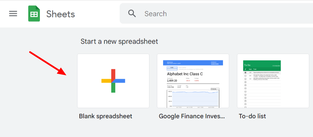
This method gives you the most control over your table's appearance. Launch the Google Sheet app or go to URL sheets.google.com. Next, click the "+" button to create a new spreadsheet.
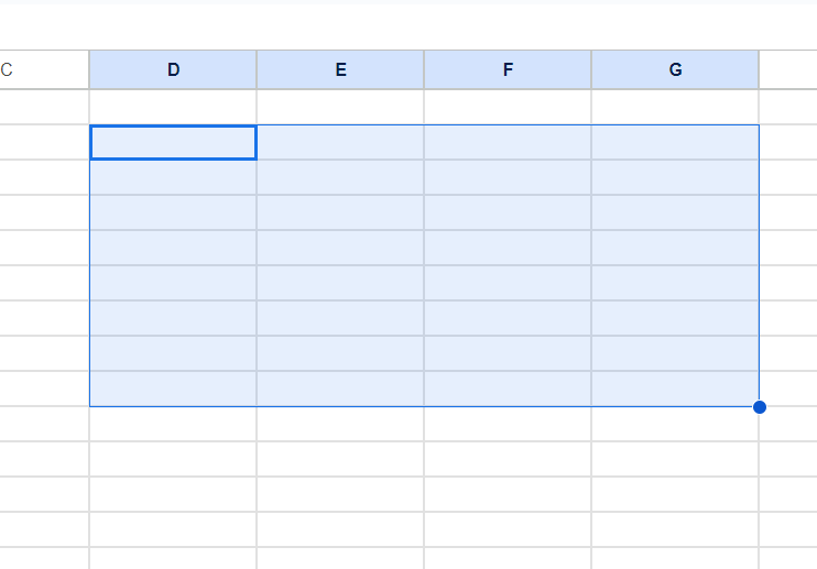
Next, select your table range. To select your table range, click on the top-left cell where you want your table to start, then drag to the bottom-right cell to encompass the entire intended table area.
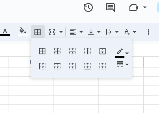
Choose border style. After selecting your cells, scroll up to the toolbar. Click the border icon (it looks like a grid) and choose your preferred border style.
Create column headers in the top row of your selected range. These describe the data each column will contain. Make them stand out by making them bold or changing their background color using the toolbar options.
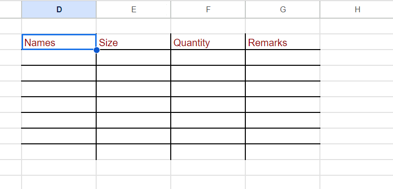
Enter your data by clicking on each cell below the headers. After entering data, use the Ctrl + Enter shortcut to move to the next cell below quickly.
Google Sheets automatically saves your work when connected to the internet. But always ensure a stable connection while working.
Method 2: Insert Option
This is a quick way to create a table with pre-designed formatting.
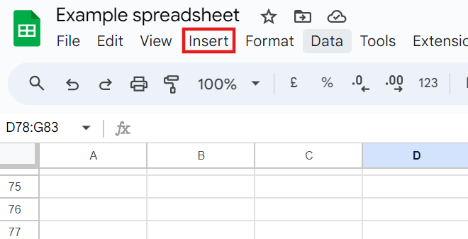
Navigate to the top menu and click "Insert.”
Choose "Table" from the dropdown menu.
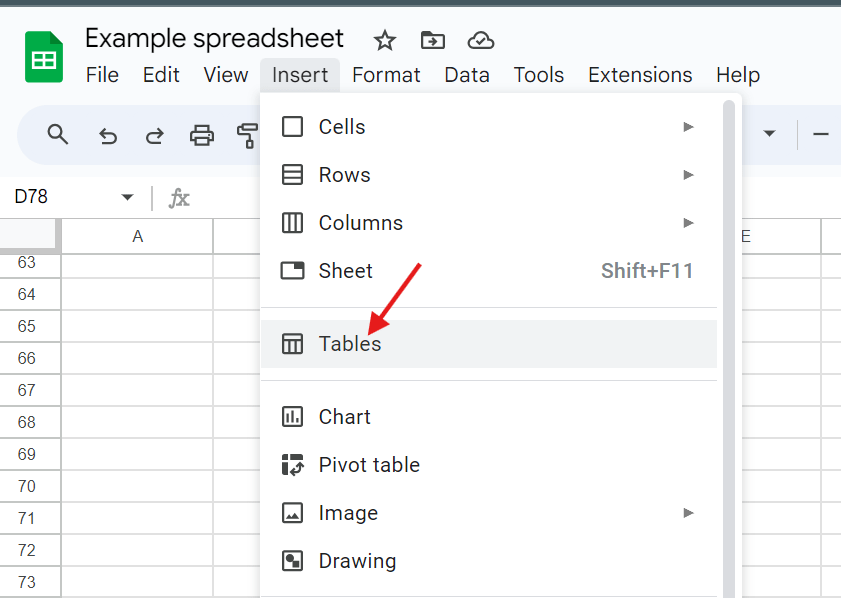
Google Sheets will present several table templates from which you can choose.
Select the one that best suits your needs. Then, you can modify the table by adding your data and adjusting the formatting as needed.
Method 3: Format Option
This method quickly converts an existing range of data into a formatted table.
Select the entire range you want to convert into a table or the range you want your table to be if you don't have existing data.
Click "Format" in the top menu.

Then select "Convert to table" from the dropdown menu.
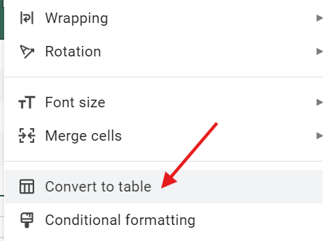
Google Sheets will automatically format your selected range as a table, typically adding borders and alternating row colors for better readability.
If you haven't already, add headers to the top row. Make them stand out by making them bold or changing their background color.
Lastly, enter your data into the cells below the headers if you haven't already done so.
Each method has advantages. The Manual method offers the most customization but requires more work. The Insert option is the fastest if you like Google's pre-designed templates. The Format option is ideal for quickly formatting existing data as a table.
Benefits of Using Tables in Google Sheets for Marketers
Tables in Google Sheets help marketers organize, analyze, and visualize data more effectively. They improve workflow efficiency and support better decision-making.
Here are some of the most important benefits of using tables in Google Sheets
1. Improve Data Organization and Analysis
Tables provide a structured format for large datasets, making information easier to find and manage. Customizable formatting and various column types reduce errors and streamline data handling. This structure allows for quicker analysis of metrics and campaign tracking.
2. Enhance Data Visualization
Tables simplify the creation of charts and graphs, making it easier to identify trends and insights. You can create visual representations directly from your data, which update automatically as the data changes. This improves how you communicate information to your team and stakeholders.
3. Simplify Data Comparison
You can use tables to organize data points side by side, making spotting trends, differences, and correlations easier. Filters and sorting functions help you focus on specific data sets for detailed comparison. Consistent column types reduce errors during analysis, leading to more accurate comparisons and better-informed marketing strategies.
4. Automate Calculations
Tables support formulas to automate calculations, reducing manual work and potential errors. Functions like SUM, IF, and VLOOKUP make managing data analysis and metric tracking easier. Google Sheets' collaborative nature also allows for real-time teamwork on these calculations.
5. Filter and Sort Data Effectively
Tables offer robust filtering and sorting capabilities, allowing you to analyze specific data segments quickly. You can apply multiple filters to refine results and sort data to identify patterns quickly. Filter views let team members customize their data display without affecting others, balancing individual needs with team collaboration.
These features help turn raw marketing data into valuable insights, supporting more effective campaigns and strategies.
How to Format a Table in Google Sheets
Once you've created your table, you can format it to enhance readability and analysis.
Here are some of the most common formatting options to implement :
Adjusting Column Width and Row Height
To resize columns or rows for better data visibility, click and drag the borders of the column or row headers.
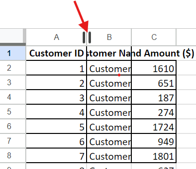
This allows you to accommodate longer text or provide more white space.
Changing Font Styles and Sizes
Select the cells you want to modify, and then use the toolbar to choose a different font and size.
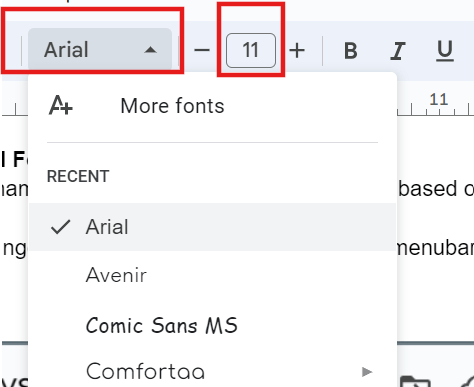
Experiment with various options to find what works best for your data presentation.
Applying Cell Colors
Highlight cells or text by changing their color. Select the area you want to modify, then use the fill color option in the toolbar to choose your preferred color. This can help categorize data or draw attention to specific information.
Using Conditional Formatting
You can create dynamic formatting rules on Google Sheets based on cell content.
Select your data range, then go to Format at the top of the menu bar.
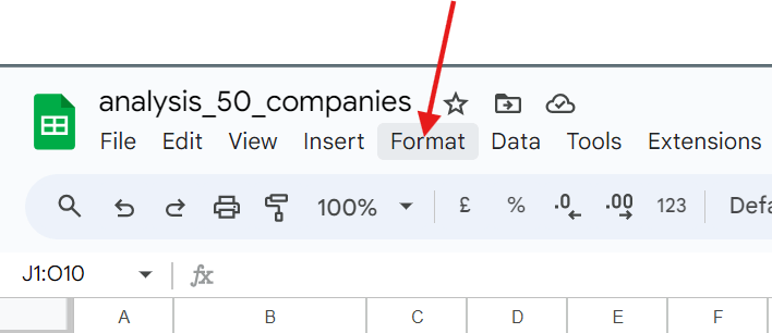
Scroll down and select “Conditional formatting”.
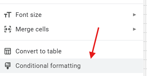
Here, you can set rules for automatic cell formatting based on specific criteria, such as highlighting all cells above a particular value.
Aligning Text within Cells
Adjust text position for better presentation using two methods:
1. Select the columns or rows you want to align, then use the alignment options in the toolbar to adjust the text position.
2. Alternatively, click 'Format' at the top of the sheet, then select "Alignment" from the dropdown menu for more detailed options.
How to Use Formulas within a Table in Google Sheets
Here's a step-by-step explanation of how to use these functions:
Using the SUM Function
To use formulas within a table in Google Sheets, particularly the SUM and AVERAGE functions, follow these steps:
Click on the cell where you want the sum to appear.
Type "=SUM(" (without quotes).
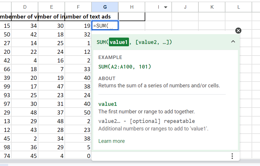
Select the range of cells you want to add up.
Close the parenthesis and press “Enter”.
AVERAGE Function
1. Click on the cell where you want the average to appear.
2. Type "=AVERAGE(" (without quotes).
3. Select the range of cells you want to average.
4. Close the parenthesis and press Enter.
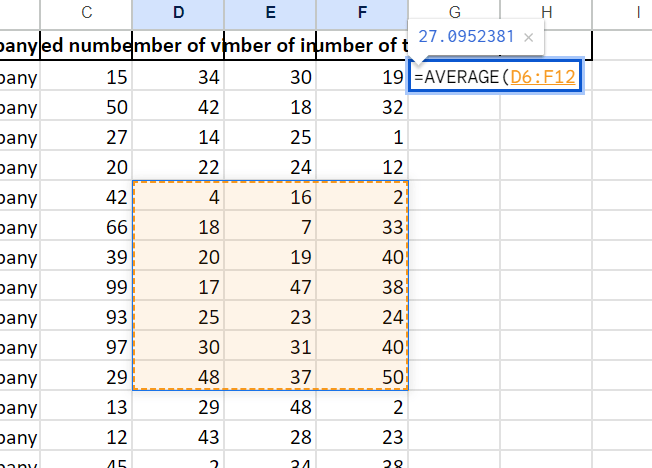
In the image example above, The formula for average values in cells D6 through F12 is =AVERAGE(D6: F12)
How to Use IF Formulas within a Table in Google Sheets
IF statements in Google Sheets are powerful tools that allow you to introduce conditional logic into your spreadsheets. They evaluate a condition and return one value if it is accurate and another if it's false.
To use IF statements within a table in Google Sheets for marketing-related scenarios, you can follow this approach:
The basic syntax of an IF statement in Google Sheets is: =IF(condition, value_if_true, value_if_false)
Here are some examples relevant to marketing:
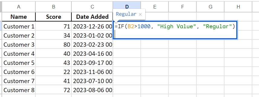
1. Categorizing customers by spend:
If you have a data list of customers and want to categorize them by spending, you don’t have to analyze the data manually.
This example categorizes customers as "High Value" if their spend (in cell B2) is over $1000 and "Regular" otherwise.
Syntax:
=IF(B2>1000, "High Value", "Regular")
2. Assigning follow-up actions based on lead score:
You can set up the IF formula to assign different marketing or sales follow-up actions based on scores, your leads, or specific parameters.
For example, Scores over 70 get immediate contact, scores between 40 and 70 get email nurturing, and lower scores are added to the newsletter.
The syntax will look like this:
=IF(B3>70, "Immediate Contact", IF(B3>40, "Email Nurture", "Add to Newsletter"))
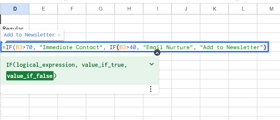
This nested IF statement assigns different actions based on a lead score in cell B3. Scores over 70 get immediate contact, scores between 40 and 70 get email nurturing, and lower scores are added to the newsletter.
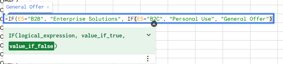
3. Tailoring messaging based on customer segment:
You can use this to formulate and select appropriate messaging based on the customer segment in any cell of your choice, choosing between B2B, B2C, or a general offer.
For example,
=IF(E5="B2B", "Enterprise Solutions," IF(E5="B2C", "Personal Use," "General Offer"))
VLOOKUP:
VLOOKUP is short for vertical Lookup and is used to search for a value in the leftmost column of a table and return a value in the same row from a specified column.
Here are ways to use VLOOKUP.
Syntax: =VLOOKUP(search_key, range, index, [is_sorted])
search_key: The value to search for in the first column of the range
range: The table or range to search
index: The column number in the range to return a value from
is_sorted: (Optional) TRUE for the approximate match, FALSE for an exact match
How to use VLOOKUP in Google Sheets
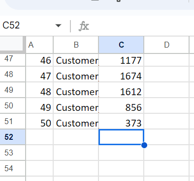
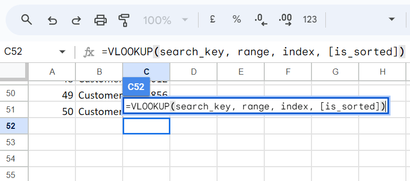
Choose the cell where you want the information you're looking for. In this example, click on cell C52.
Next, enter the VLOOKUP formular into that cell: =VLOOKUP(search_key, range, index, [is_sorted])
When to use VLOOKUP:
Best for tables where categories are in the leftmost column
Useful when you need to find corresponding data in columns to the right
HLOOKUP
HLOOKUP (Horizontal Lookup) is a function in Google Sheets that searches for a value in the top row of a table and returns a value in the same column from a row you specify.
The formula works with horizontally organized data, such as a table with your categories in the top row and the corresponding data in the rows below.
Syntax: HLOOKUP(search_key, range, index, [is_sorted])
Here's how to use it:
search_key: The value you're looking for in the first row of the table
range: The table or array you want to search
index: The row number in the range from which to return a value
is_sorted: (Optional) TRUE if the first row is sorted, FALSE if not. The default is TRUE.
Example:
Let's say you have a table with different product information.
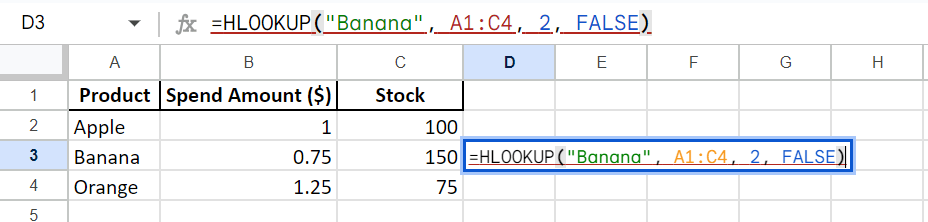
To find the price of "Banana": =HLOOKUP("Banana", A1:C4, 2, FALSE)
This would return 0.75.
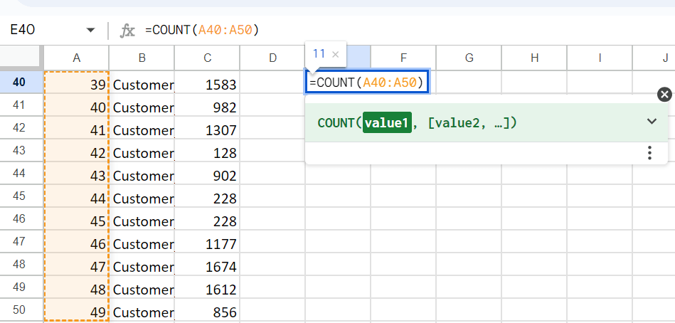
COUNT and COUNTA
The COUNT and COUNTA functions in Google Sheets are used to count cells within a specified range, but they differ in the types of data they count.
Let’s look at each function and their differences:
COUNT Function:
Counts only cells containing numerical values within the specified range.
Ignores empty cells, text, logical values (TRUE/FALSE), and error values.
Syntax: =COUNT(range1, [range2, ...])
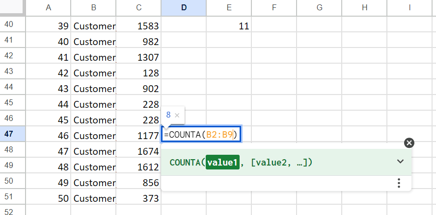
COUNTA Function:
Counts all non-empty cells within the specified range.
Includes cells containing numbers, text, logical values, dates, and error values.
Only ignores empty cells.
Syntax: =COUNTA(range1, [range2, ...])
For Example,
Key differences between COUNT and COUNTA
1. Scope of counting
COUNT: Tallies only numerical values
COUNTA: Includes all non-empty cells (numbers, text, logical values, dates, errors)
2. Optimal applications
COUNT: Best suited for numerical data such as quantities or scores
COUNTA: Preferred for tallying all populated cells, regardless of content type
3. Treatment of non-numerical data
COUNT: Excludes text and logical values
COUNTA: Incorporates text and logical values in the tally
Your new AI Data Analyst
Extract from PDFs, import your business data, and analyze it using plain language.
Try Rows (no signup)How to Use Rows to Supercharge Your Sheets
Rows is a comprehensive spreadsheet for modern teams that offers better UX for data ingestion and has native AI capabilities (AI analyst, AI-generated subtitles, native AI functions).

Below are a few simple steps to follow when creating a table in Rows:
Step 1: Open a new spreadsheet on Rows.com. You can do it just by visiting Rows homepage: you will land right away on a full-working spreadsheet. No account needed.
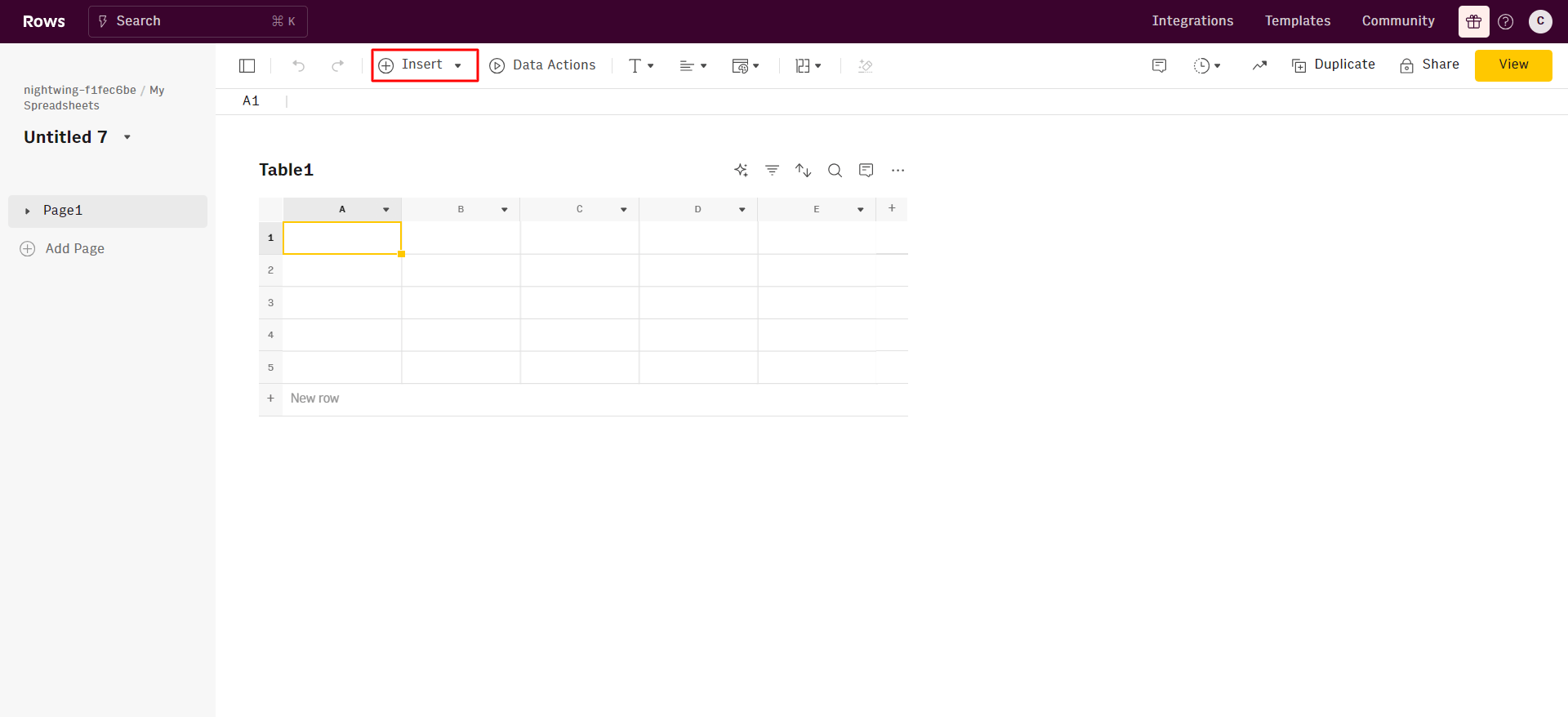
Step 2: To insert a new table you can click the “insert” menu and choose “Table”. Once done, you'll see a new table added to your workspace.
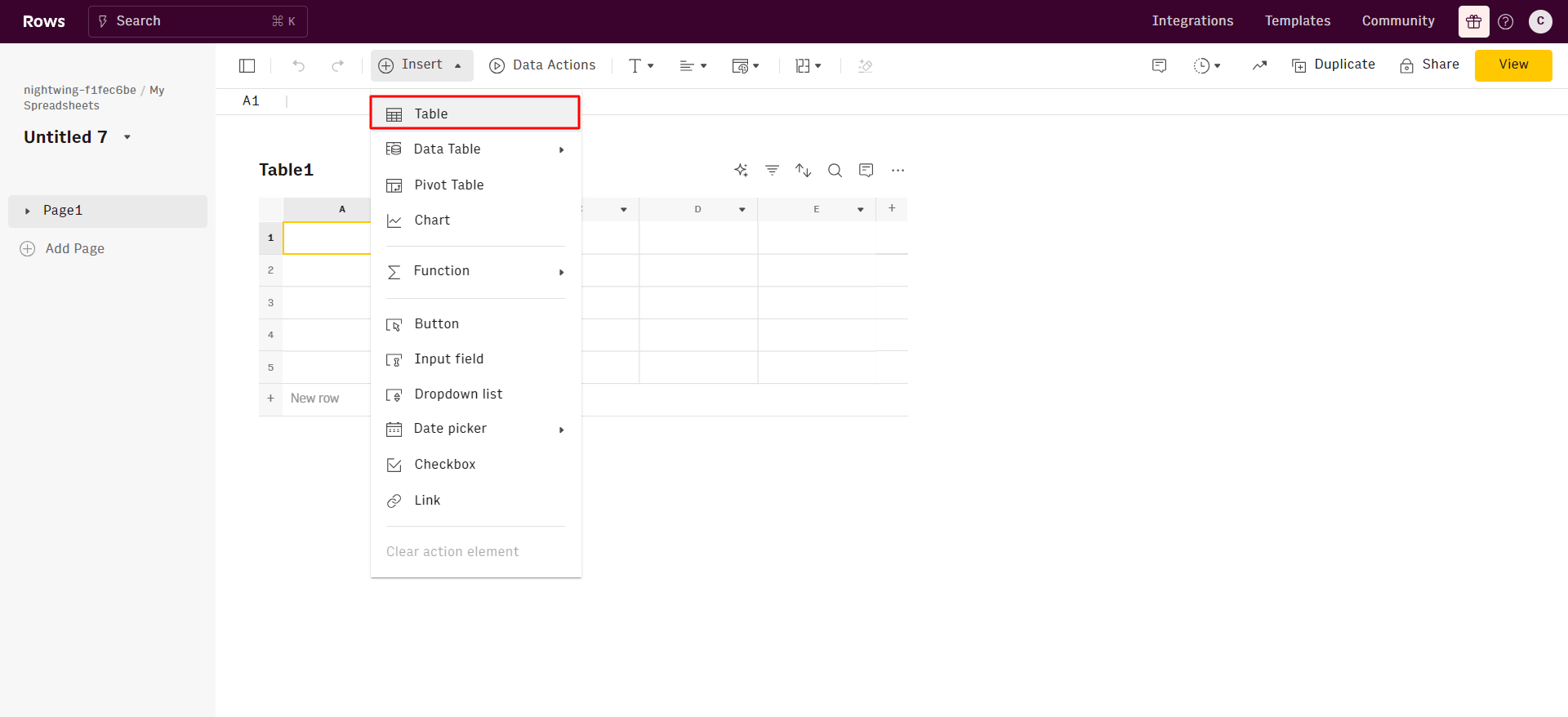
Alternatively, you can click on the + icon next to each table: a simple click will open a new table below the selected one, while option-click will add it above. In Rows you can add a Table (regular one, empty by default) or a Data Table, a table that is connected to an external data source. See the next paragraph to know more about how to ingest live data on your spreadsheet.
Step 3: What is a table without data? After creating a table, import data from a CSV file or of our Rows built-in data integrations. See the following example:
How does Rows compare with Google Sheets for creating tables?
Rows has many advantages over Google Sheets when it comes to creating tables. Let's take a look at these benefits:
Modern UI
Rows has a tidier UI when compared to Google Sheets. Here are features that make its UI clear off:
Spreadsheets in Rows present a document-like layout with standalone tables and charts that are stacked vertically and horizontally.
WYSIWYG: the spreadsheet IS the dashboard. All data is rendered as regular spreadsheet tables. And you can move elements vertically and horizontally with drag&drop.
View Mode: View mode transforms your spreadsheets into web applications. Thanks to input fields you can help anyone interact with your spreadsheets and gather all the insights error-proof. See the example below:
Embed feature
You can use the Embed feature to showcase your Rows’ tables and charts inside Notion, Confluence or any other tools that support iframes. You can embed any element from a spreadsheet - a Table, Chart, or Form - and have a live connection between your Notion doc and Rows spreadsheet.
Choose Embed in the settings menu in the right-hand corner of the element you want to embed.
Click the Share Privately toggle.
Click Copy link
Paste the link on a Notion doc and click to Create embed
50+ built-in data source integrations in various domains
Rows boast over 50+ integrations across different facets like marketing, data warehouse, etc.
This makes it easy to ingest data into your table quickly and reduces your team's stress. With Rows, you can gather data from various sources in your system. This allows for more detailed analyses and helps your team uncover insights they might miss.
Here's a division of the built-in integrations in Rows:
Marketing: GA4, GSC, Facebook, Instagram, Tiktok
Productivity software: OpenAI, Notion, Slack, Email, Translate
Data warehouse: MySQL, BigQuery, PostgreSQL, Snowflake, Amazon Redshift
Read more: Best data aggregation tools in 2025.
AI-powered automation
With the AI Analyst, you can ask AI to analyze, summarize, transform, and enrich your analysis. Click on the ✨ icon, at the top right corner of any table.
A chat interface will open on the right: you can ask a broad range of questions, from basic spreadsheet commands - plotting a chart or adding or formatting columns - to more complex tasks, such as slicing, pivoting, or computing metrics about your data.
For example, given a dataset with daily revenue and costs of various marketing campaigns, you can ask the Analyst to add a column with the profit margin. Watch the video below:
In addition, our AI Analyst is instructed to use our native OpenAI functions to perform data enrichment or extraction tasks.
For example, you can ask the AI analyst to run a sentiment analysis on a column with product reviews, or add a column that categorizes addresses into regions, see below:
Want to know more about how our Analyst works? Check out our guide or watch our demo.
Your new AI Data Analyst
Extract from PDFs, import your business data, and analyze it using plain language.
Try Rows (no signup)Related: Do you want to learn how to create pivot tables? If yes, click the link!
Learn more about Rows’ AI analyst
Start using Rows today!
With Rows, you get an AI analyst that automatically derives insights from multiple tables as you want. The Analyst slices the main table by highlighting the top keywords by clicks.
Ready to get started with Rows.com? Start using the product right away for free.