The filter button  is great for filtering entire tables. But what if you want to filter only a subset of the table?
For example, maybe you want to filter the “price” column by a certain price range but only for rows where the product column contains “iPhone”.
In complex cases like this, it’s often better to use a formula to construct your filter query rather than relying on the user interface. That’s where the FILTER function comes in handy.
You can use the FILTER function to filter data in a normal table or in a {data} cell.
In this guide, we’ll show you:
- the arguments for the
FILTERfunction, - example FILTER use cases,
- how you can use
FILTERin combination with theFILTER_COLUMNSfunction.
Try it Yourself
Using the FILTER function
The easiest way to get started with the FILTER function is through the Function Wizard.
To use the FILTER function with the Function Wizard, follow these steps:
- Select a cell adjacent to a column or table that contains several rows of data.
- Underneath this cell should be enough free space to insert copies of the formula.
- Underneath this cell should be enough free space to insert copies of the formula.
- Click the Actions
 button in the main toolbar.
 - In the search box, search for "FILTER" and click the result.
- In the options panel, configure the options for the
FILTERfunction.
| OPTION | USE TO |
|---|---|
| Data | Define the data that you want to filter. This value could be:‘Table1’!A1:F50 A1 |
| Condition | Define the data that you want to filter on. This value could be:F1:F50 (single column) [“year”]You can combine conditions with * (AND) and + (OR).For example: (A1:A5>5)*(A1:A5<10)If you get the error: “The condition should have a range or JSON data with the same height or width as data.”, make sure that the range has the same number of rows or columns as the range in the Data field. </li></ul> |
| Set if Empty (optional) | Define a custom message to display when there are no matching results. The argument allows you to add a more human-readable message when no match is available (instead of just showing a blank cell).
|
| Set Mode | Change how the first row is treated. Possible values are 1 and 0: |
Filtering Examples
To get a better idea of how this function works, check out the following examples:
Filter for specific values in a column
Let’s say you’re analyzing some Google Analytics data and you notice some outliers that you don’t want to show up in your report. Here’s an example of a Google Analytics Table.
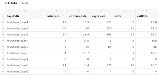
Here we want to filter for web pages where the exit rate falls within a realistic range, such as between 10% and 75%. We also want to make it easy to change the range, so we can experiment with different ranges.
It would be easier if we could put the minimum and maximum range in cells and have the filtered view update automatically whenever we change those cells.
You could put these criteria in a dedicated “FilterCriteria” table, like this:
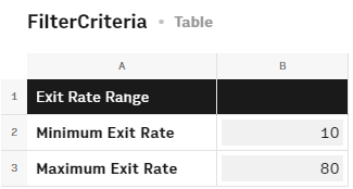
That's what makes the FILTER function so useful. With the FILTER function, you can refer to other cells.
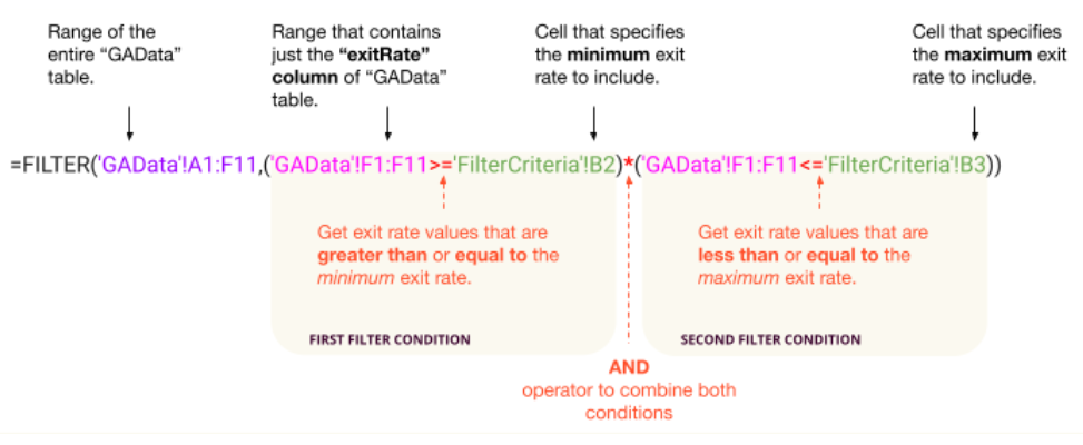
To filter for Exit Rates in a specific range, using the values in our FilterCritera table, we could use the following FILTER formula:
=FILTER('GAData'!A1:F11,('GAData'!F1:F11>='FilterCriteria'!B2)*('GAData'!F1:F11<='FilterCriteria'!B3))
Here’s a breakdown of how it works:
When you enter this function, you’ll get a {data} cell, rather than a filtered table.
To see the resulting data in a table:
- Use an
OVERWRITEformula to generate a table from the {data} cell. For example, if you entered theFILTERformula in ‘A1’, you could enter the following inA2:=OVERWRITE(A1) - Create a Data Table from the {data} cell.
Click the cell actions button
 to open the Cell Actions menu and select Create Data Table
The resulting table should resemble the following example:

We now only have rows where the exit rate falls within the range that we specified in our "FilterCriteria" table.
Filtering data in a {data} cell
In our previous examples, we’ve been filtering data in a source table to create a second filtered version of that table.
However, if you’re using integration functions to get external data, you don’t need a source table. You can filter the raw data in the {data} cell, and create a table from the filtered result—so one less table to worry about.
Here’s an example:
- Let’s say you’re using the
SEARCH_COMPANIESfunction to get a list of Berlin-based venture capital firms with more than 50 employees. - Here’s how the formula would look:
=SEARCH_COMPANIES(">50","Berlin","Venture Capital & Private Equity") - The result is returned in a {data} cell that looks like this:

If you view the data you’ll see that there are a number of interesting attributes to filter on—for example, the year that the VC was founded.
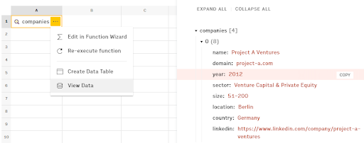
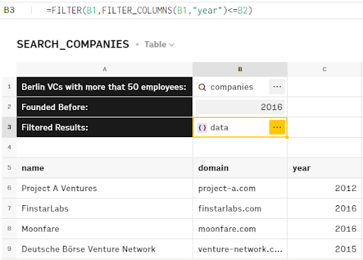
Let’s say we want to narrow this list down to VCs that were founded before 2016. In this case, we would enter the filter formula like so:
=FILTER(B1,FILTER_COLUMNS(B1,"year")<=2016)
- Note that the formula includes a
FILTER_COLUMNSfunction. We’ll explain this function more in the final section. - For now, it’s enough to know that we’re using this function to indicate which parameter we want to filter on (in our raw data, parameters serve the same purpose as columns in a table—they store data that falls into a specific category such as years).
Now we can go further, and put our filter criteria in a separate cell like last time. In the following example, we’ve put it, the FILTERformula in B3 and referenced the cell above it for the filter criteria (B2).
Filtering columns by column name
The FILTER_COLUMNS function gives you a way to isolate specific columns that you want to work with. For example, let’s say you’re working with Google Analytics report but you’re only interested in Bounce Rate.
Your visitor report table might contain a lot of metrics like “visits”, “%New Visits”, and so on. However, you want to get a view that includes only the columns that you’re interested in.

You can create a simpler version of this table by filtering for just the relevant columns.

To render the data as a table, you can then nest this formula one of the INSERT(), OVERWRITE(), or UPDATE() functions like this: =OVERWRITE(FILTER_COLUMNS('All Data'!A1:H100,'["Page","Bounce Rate"]'))
Which produces a much cleaner looking table:

By the way: if, for some reason, you’re annoyed by the table headers, you can omit them from the formula result.
- To omit the table headers, add an optional
FALSEargument to the filter formula, like this:=FILTER_COLUMNS('All Data'!A1:H100,'["Page","Bounce Rate"]',FALSE)
Further Reading
As useful as FILTER and FILTER_COLUMNS are, sometimes you need even more flexibility. Fortunately, there are more advanced methods for parsing and filtering the contents of {data} cells in particular.
To learn more about these methods, check out the following articles: