How to Add Date in Google Sheets [2025]

Adding dates in Google Sheets is super important if you want to keep tabs on your leads and sales. It might seem simple, but many people struggle with inconsistent date formatting and time zone discrepancies.
Our 2025 guide covers updated methods to help you and your team:
Use date functions in Google Sheets
Apply dates to organize lead generation funnels
Solve common date-related problems and their solutions
No worries if you're a total newbie to Google Sheets or just looking to improve your skills; you'll learn how to use dates in Google Sheets to better manage your sales and lead generation.
How to Add Date in Google Sheets Using Basic Formulas
The basic formula for the “add a date in Google sheet” is (=TODAY(), =NOW()).
Here is how to add dates in Google Sheets Using Basic Formulas
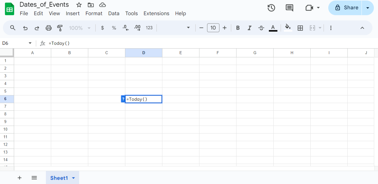
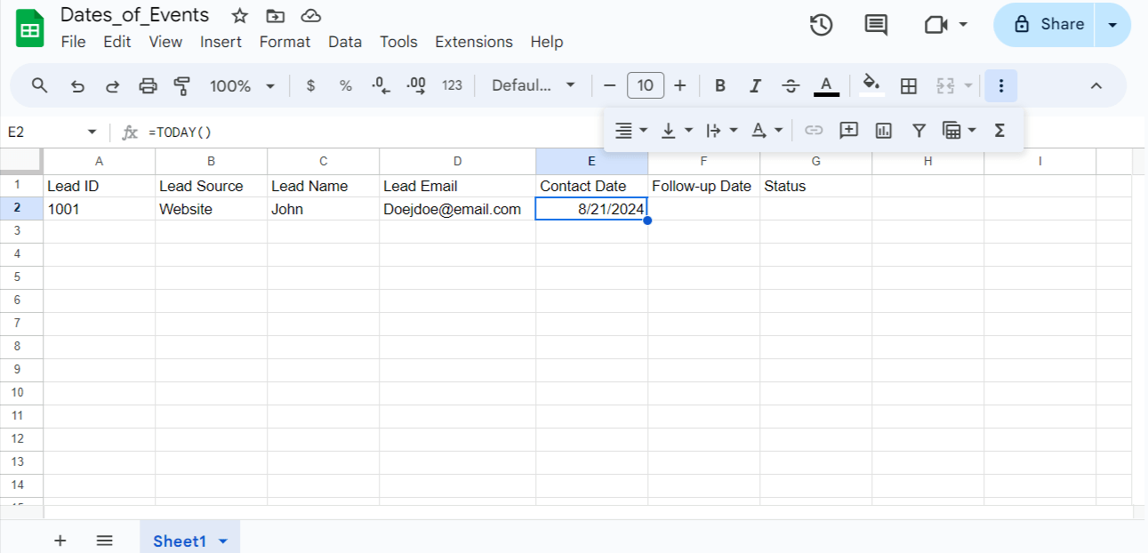
First, open your Google Sheets template. Position your cursor on the cell where you wish to insert the date; type =TODAY(). Press the Enter key for the result.

The spreadsheet for modern teams
Save hours on data import, surface insights by asking, and share beautiful, ready-to-use dashboards.
Get Started (free)Manual Entry vs Automatic Date Functions in Google Sheets
Google Sheets offers two primary methods for adding dates: manual entry and automated date functions like =TODAY() or =NOW(). While both can achieve the same result, each approach has distinct advantages and drawbacks.
Let's take a look at the pros and cons of both methods to help you decide.
Manual Date Entry
Pros:
Offers greater flexibility in date formatting
Allows for easy input of past or future dates
Doesn't require formula knowledge
Maintains static dates that won't change unexpectedly
Cons:
Increases the risk of human error
It can be time-consuming for large datasets
Requires manual updates if dates need to change
May lead to inconsistent formatting across entries
Automated Date Functions
Pros:
Automatically updates dates, reducing errors
Ensures consistency across all entries
Saves time when working with current dates
Easily adjustable for different time zones
Cons:
Requires some technical knowledge to set up correctly
It may not be suitable for historical or future date entries
It can cause unexpected changes if formulas are altered
Might need additional formatting to display dates as desired
Using the TODAY and NOW Functions
TODAY() and NOW() are two nifty functions on Google Sheets that you and your team can use to keep track of dates and times. These functions automatically update to reflect the current date or date and time, eliminating the need for manual updates. Here's how you can put them to work:
1. Using =TODAY()
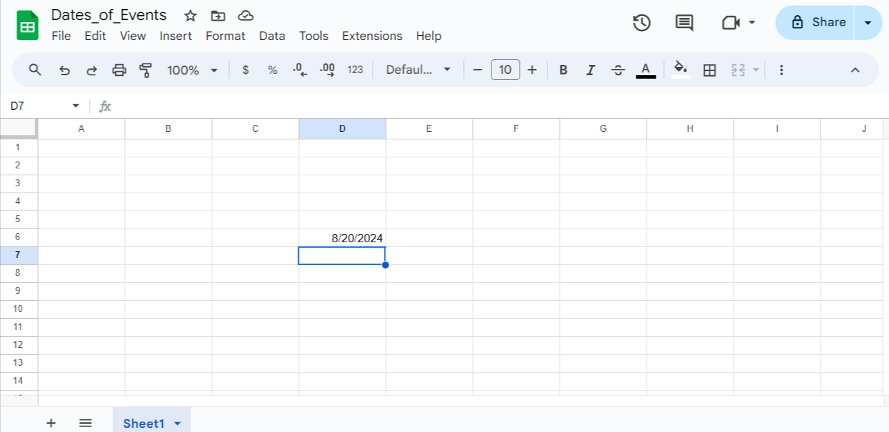
The =TODAY() function will insert the current date into the selected cell.
For example, typing =TODAY() in a cell will display the current date, such as "8/20/2024".
This date will automatically update each time you open or refresh the Google Sheet, reflecting the current date.
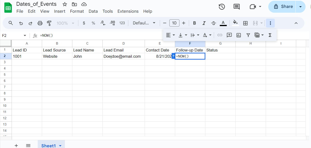
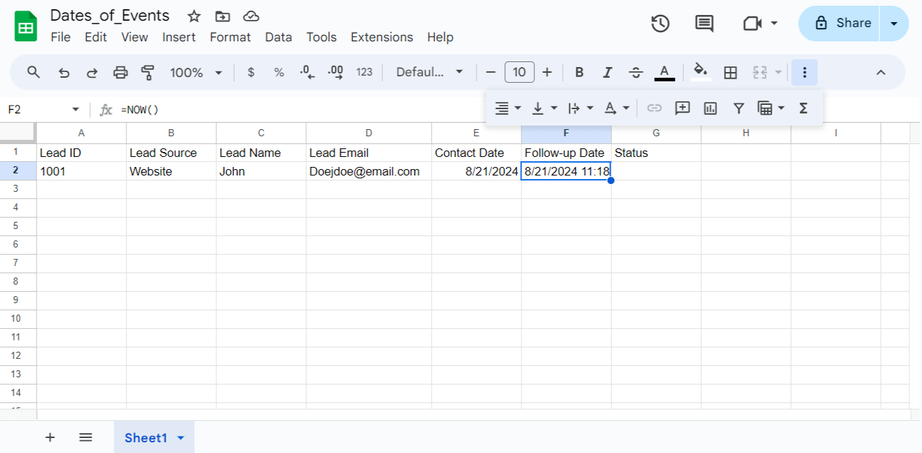
2. Using =NOW()
The =NOW() function will insert the current date and time into the selected cell.
For example, typing =NOW() in a cell will display the current date and time, such as "8/20/2024 12:34:56 PM".
Like =TODAY(), the date and time will automatically update each time you open or refresh the Google Sheet.
Adding Conditional Formatting Based on Dates
Adding conditional formatting based on date offers several key benefits for effective lead management. Some of these include:
Identifying aging leads quickly and
Optimizing lead nurturing
Here are the steps to use conditional formatting in Google Sheets to visually highlight leads based on their date data.
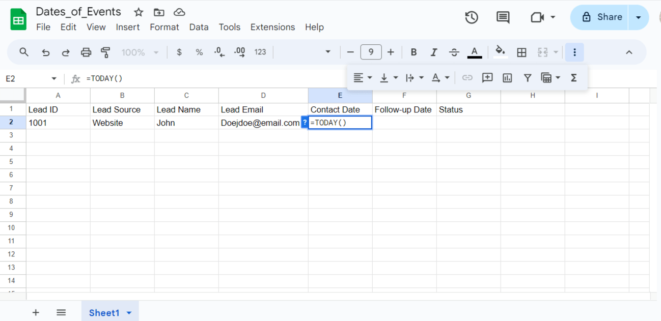
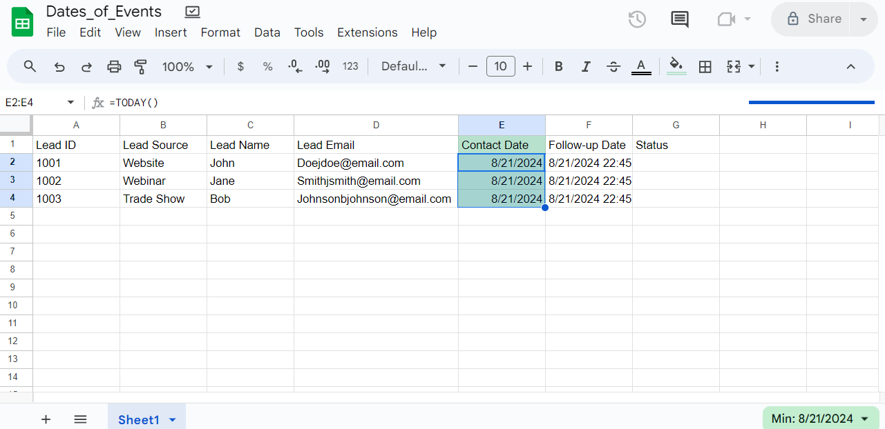
Step1: First Set up the Lead Generation Tracking Sheet (see sample below)
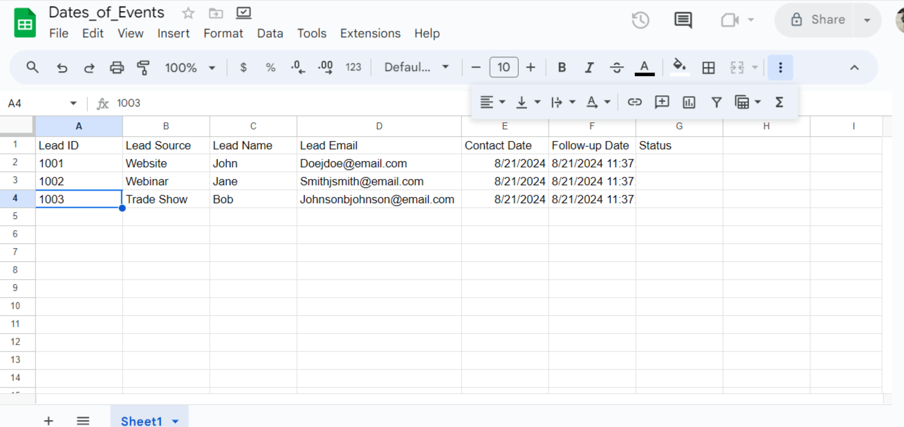
Step 2: Identify the relevant date column. This is to help highlight leads that have aged beyond a certain period. In this case, we use the “Contact Date” column.
Step 3: Apply conditional formatting
Select the Contact Date column. Next, navigate to the menu bar and click the "Format" menu.
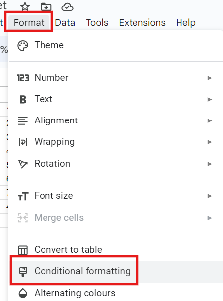
Then pick "Conditional formatting".
Step 4: Define the conditional formatting rules
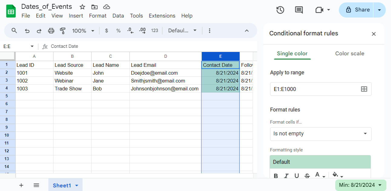
The "Conditional Formatting" dialog on the right helps you create rules to highlight cells based on certain criteria.
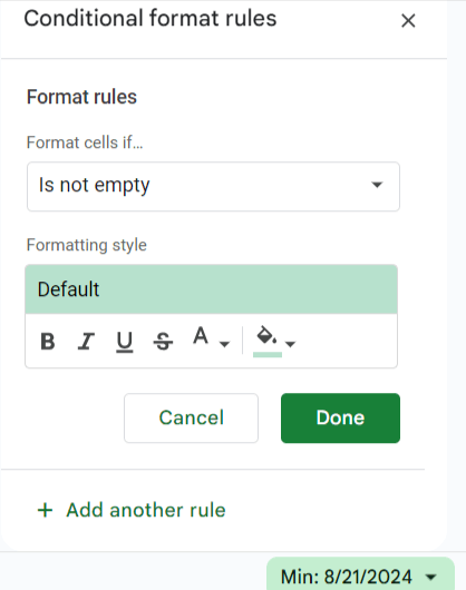
For example, to highlight leads that are old after a specific date, click the “Add another rule" button at the bottom of the conditional format dialogue box.
For the "Format cells if" condition, choose "Date is after".
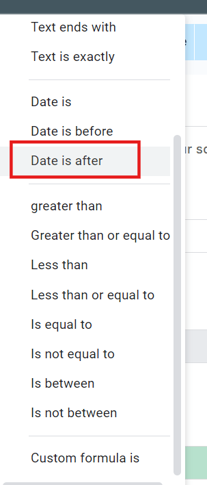
Then, enter your specific date.
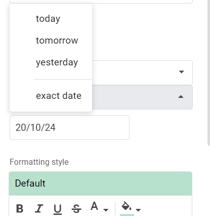
You can proceed to customize. Select the desired formatting, such as changing the cell background color or applying a bold font.
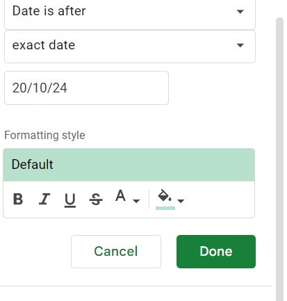
Click "Done" to apply the rule.
Common Issues When Adding Dates in Google Sheets and How to Fix Them
Incorrect Date Formatting
The date is displayed in a format that doesn't match your preferences or organizational standards.
Here’s how to solve incorrect date formatting
Select the cell(s) with the date.
Go to the "Format" menu and choose "Number".
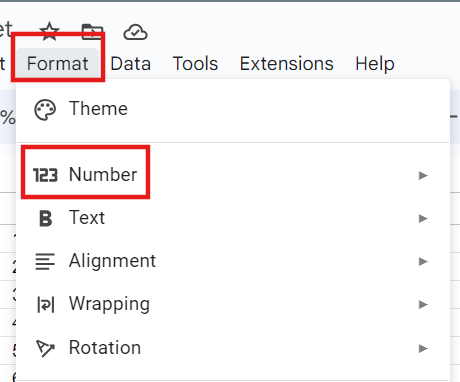
Select the desired date format, such as "Date", "Date time", or a custom format.
Adjust the column width if the date is not fully visible.
2. Time Zone Discrepancies
Sometimes, the date and time displayed in your Google Sheet do not match the local time zone.
Here’s how to solve for time zone discrepancies:
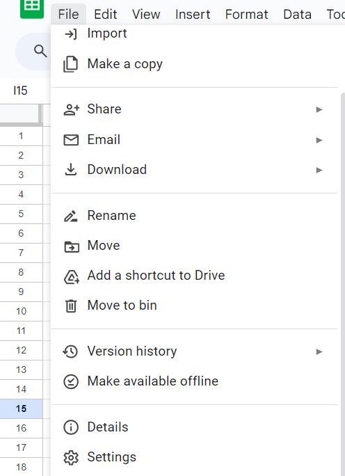
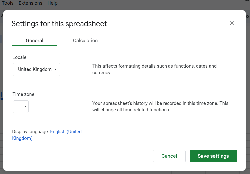
Go to the "File" menu and select "Settings".
In the "Settings" window, locate the "Time zone" section.
Select the appropriate time zone from the dropdown menu.
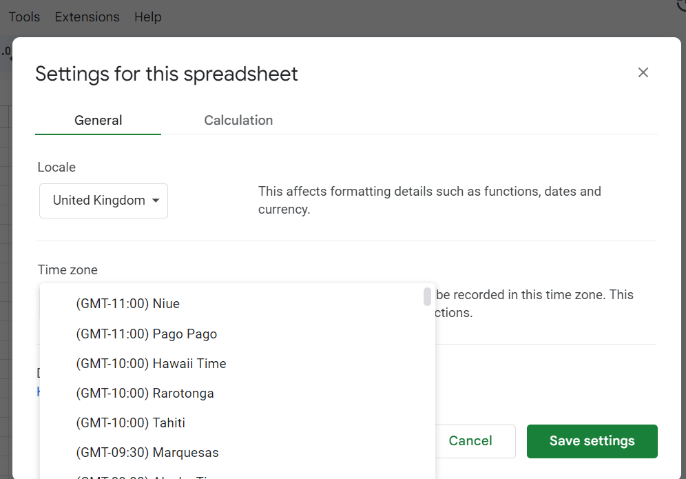
Click "Save settings" to apply the changes.
3. Incorrect Date Calculations
The date calculations (e.g., =TODAY()+7, =DATEDIF()) are not producing the expected results.
Step 1: Verify the date format in the cells you use for the calculation.
Step 2: Check the syntax of the date function you're using (e.g., =TODAY(), =DATE(year, month, day)).
Step 3: Ensure that the referenced cells or date values are in the correct format (e.g., not as text).
Use the =VALUE() function to convert a text-formatted date to a numeric date value before calculating.
4. Unexpected Date Updates:
Sometimes, the date in a cell automatically updates when you least expect it. Here’s how you can prevent this issue.
Confirm that you're using the appropriate date function (e.g., =TODAY() for the current date, =NOW() for the current date and time).
If you want to prevent the date from automatically updating, you can copy the cell with the date and paste it as "Values" instead of "Formulas".
Alternatively, you can convert the date formula to a static value by selecting the cell and pressing Ctrl+Shift+V (Windows) or Cmd+Shift+V (Mac)
Handling Daylight Saving Time (DST) Changes
Daylight Saving Time changes can leave you with incorrect time. To prevent this issue, ensure that the time zone setting in your Google Sheets is correct (See the steps in how to solve for time zone difference above).
If you're using date functions like =TODAY() or =NOW(), the dates should automatically adjust for Daylight Saving Time changes.
If you're manually entering dates, double-check that the date is correct, especially around the start and end of Daylight Saving Time.
Fixing Incorrect Date Formats
Here are some best practices and solutions to address incorrect date challenges:
Use ISO 8601 Date Format
If you’re working with teams or collaborating on a project on Google Sheet, it’s best to adopt the ISO 8601 date format (YYYY-MM-DD) as a universal standard.
This format eliminates ambiguity between different regional date formats and prevents discrepancies.
For example, 2024-08-22 instead of 08/22/2024 or 22/08/2024
How to Use Google Sheets’ Built-in Date Formatting to set a consistent format.
First method: Use Format option in the menu bar.
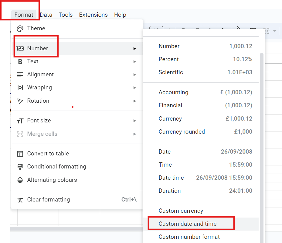
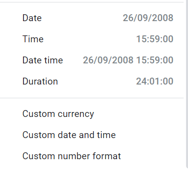
Go to Format, scroll to Number and click “Custom date and time”.
Next, use custom number formatting for more control. Create a custom format that works for all regions, e.g., "yyyy-mm-dd".
Second method: Use the DATE() Function
Input dates using the DATE() function: =DATE(year, month, day). This approach is less prone to regional misinterpretation.
How to Standardize Time Zones in Google Sheets
You can adjust the setting on Google Sheets to set up a uniform time zone on Google Sheets.
Here’s how it works.
Step 1: Click file, scroll over to setting and click.
This will open an option to customize time zone.
Step 2: Select your preferred time zone.
Handling Time Zone Discrepancies in Google Sheets
Time zone differences can wreak havoc on your data consistency and team coordination especially when you’re when you're working with a global team or customer base.
Let's break down the most common time zone issues you might face and how they can impact your workflow:
1. Inconsistent Lead Capture Times:
Users in different time zones may record lead capture times based on their local time, leading to discrepancies in the actual order of lead acquisition.
2. Misaligned Follow-up Schedules:
"Let's follow up tomorrow" sounds simple, right? Not when your "tomorrow" is someone else's "today" or even "yesterday". A follow-up scheduled for "tomorrow" might mean different things to team members in various time zones, resulting in delayed or premature outreach.
3. Reporting Inaccuracies:
When generating reports spanning multiple time zones, data can be skewed if not properly normalized, leading to incorrect performance analyses.
4. Meeting Scheduling Conflicts:
Arranging meetings or calls with leads across time zones can be challenging if the time zone differences are not clearly communicated or understood.
5. Data Sorting Issues:
When sorting leads by date and time, inconsistent time zone recording can lead to an incorrect chronological order.
Tips for Ensuring Consistency When Setting Date and Time In Google Sheet
Choose a standard time zone
For example, a popular choice for distributed teams is UTC. You can use formulas to convert UTC to local time for display purposes.
Formula:
=UTC_TIME_COLUMN + TIME(timezone_offset, 0, 0)
Use ISO 8601 Format
Adopt the ISO 8601 date-time format (YYYY-MM-DDTHH:MM:SSZ) for all records. This format includes the time zone offset, ensuring clarity.
Create a Time Zone Column:
Add a separate column to record the time zone for each lead. This allows for easy conversion and interpretation of times.
Implement Data Validation:
Set up data validation rules to ensure time entries include time zone information.
Use Google Sheets' Built-in Date-Time Formatting:
Use Format > Number > Date time to ensure consistent display across users.
The spreadsheet for modern teams
Save hours on data import, surface insights by asking, and share beautiful, ready-to-use dashboards.
Get Started (free)How to Add Date in Rows [Easier Alternative]
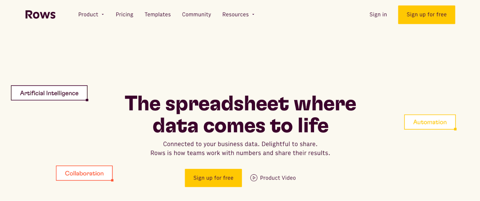
Rows is a comprehensive spreadsheet for modern teams that offers a modern UI, built-in integrations for live data ingestion, and native AI capabilities (AI analyst, AI-generated subtitles, native AI functions).
With Rows, you can add dates to your documents with ease, here's how to do it:
Step by step guide on how to use the NOW and TODAY function in Rows
The functions in Google Sheets are also applicable in Rows. The difference is that you get a modern UI, and access to AI-automation features to supercharge your spreadsheet.
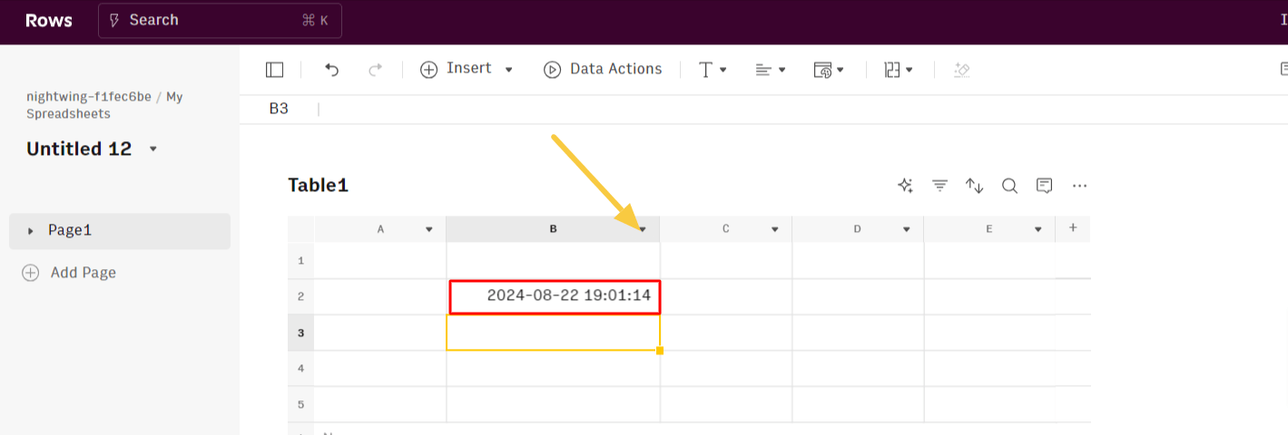
Step 1: Using NOW()
The NOW() function will insert the current date and time into the selected cell.
For example, typing =NOW() in this cell below displays 2024-08-22 19:01:14.
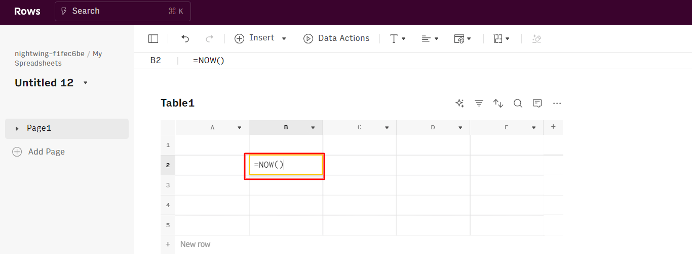
However, you have to wrap the date and time because it spills over as a result of long strings —
Click here to learn how to wrap text in Rows.
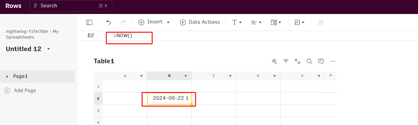
Below is the result after you wrap the result. It’ll show you the current date and time fully.
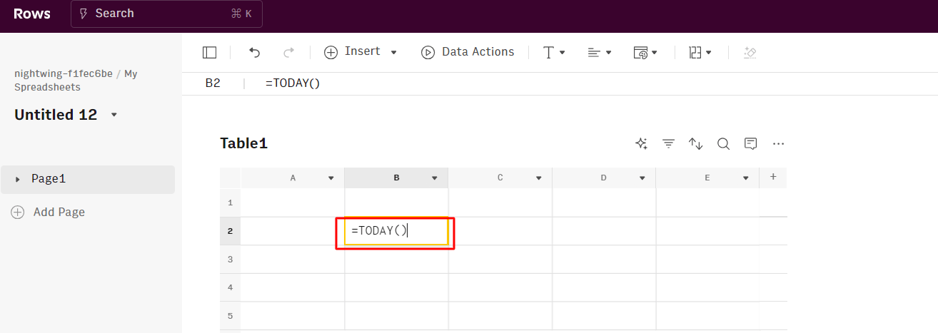
Step 2: Using TODAY()
The TODAY() function will insert the current date into the selected cell.
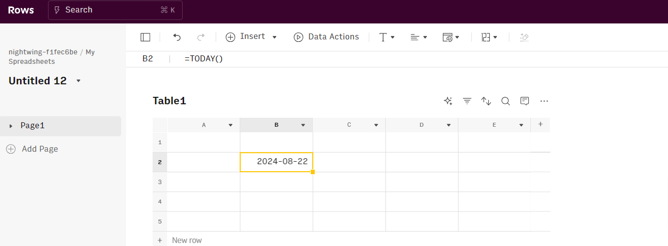
For example, typing =TODAY() in a cell will display the current date, such as "8/22/2024".
This date will automatically update each time you open or refresh the sheet, reflecting the current date.
Resulting in:
The spreadsheet for modern teams
Save hours on data import, surface insights by asking, and share beautiful, ready-to-use dashboards.
Get Started (free)Top features of Rows compared to Google Sheets
Rows has some top features that makes it an easier and better alternative to Google Sheets.
Data aggregation — OpenAI integration
You can aggregate live data from 50+ sources in a very simple manner, thanks to built-in data integrations in various domains:
Marketing: GA4, GSC, Facebook, Instagram, TikTok, etc
Productivity software: OpenAI, Notion, Slack, Email, Translate
Data Warehouse: MySQL, BigQuery, PostgreSQL, Snowflake, Amazon Redshift
And many more.
See the example below, showing how quickly you can import Google Search Console data from your account on your spreadsheet.
AI-powered automation — Helps you automatically generate averages
With the AI Analyst, you can ask AI to analyze, summarize, transform, and enrich your analysis. Click on the "AI Analyst“ ✨ icon, at the top right corner of any table.
A chat interface will open on the right: you can ask a broad range of questions, from basic spreadsheet commands - plotting a chart or adding or formatting columns - to more complex tasks, such as slicing, pivoting, or computing metrics about your data.
For example, given a dataset with daily revenue and costs of various marketing campaigns, you can ask the Analyst to add a column with the profit margin. Watch the video below:
In addition, our AI Analyst is instructed to use our native OpenAI functions to perform data enrichment or extraction tasks.
For example, you can ask the AI analyst to run a sentiment analysis on a column with product reviews, or add a column that categorizes addresses into regions, see below:
Want to know more about how our Analyst works? Check out our guide or watch our demo.
The spreadsheet for modern teams
Save hours on data import, surface insights by asking, and share beautiful, ready-to-use dashboards.
Get Started (free)Modern UI
Spreadsheets in Rows present a document-like layout with standalone tables and charts stacked vertically and horizontally.
WYSIWYG: the spreadsheet IS the dashboard. All data is rendered as regular spreadsheet tables. You can move elements vertically and horizontally with drag and drop. And if something breaks, you can intervene on that table or chart flexibly, without the need to dive into complex workflows.
View Mode: View mode makes your spreadsheets work like web applications. With input fields, you can help anyone understand how to use your spreadsheet by highlighting the cells that need an input by the user.
Supercharge your sheets with Rows
With Rows, you get access to 50+ built-in data source integrations in various domains.
This makes it easy to ingest data into your table quickly and reduces your team's stress.
With Rows, you can gather data from various sources in your system. This allows for more detailed analyses and helps your team uncover insights they might miss.
Ready to get started with Rows.com? Start using the product right away for free.