How to Calculate and Use Averages in Google Sheets in 2026 (Jan Update)

Manually calculating averages in documents like sales reports and expense reports can be time-consuming. This can leave you drowning in numbers, unable to make sense of the trends and insights buried in your financial data.

But, with the AVERAGE formula in Google Sheets, you can quickly analyze your data with just a single click.

In this guide, we will walk you through step-by-step instructions on how to use the AVERAGE, AVERAGEIF, and other average formulas in Google Sheets. From basic calculations to more advanced applications, you'll learn how to automate your average computations, visualize your findings, and optimize your workflow for better results.

What is the Google Sheets Average Formula?

The Google Sheets average function is used to calculate the mean value of a set of numbers. It is particularly useful when you need to find the central value of a range of data points, such as student grades, sales figures, or any other numerical dataset.

For example:

• Student grades: If you have a list of grades and want to find the average score.

• Sales data: Calculating the average monthly sales to assess performance.

• Budgeting: Finding the average spending across different categories.

Syntax and format:

=AVERAGE(range)

range: This group of cells contains the numbers you want to average.

Example:

Imagine you have sales data for six months in cells A1 to A6 and want to calculate the average monthly sales. You would enter the following formula:

=AVERAGE(A1:A6)

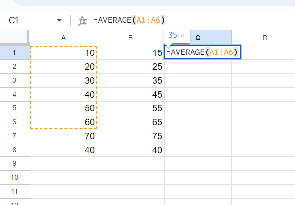
This formula will calculate the sum of the numbers in the specified range and then divide it by the number of cells in that range, giving you the average value.

Using the average function simplifies finding the mean value in your data, making it a fundamental tool in any basic spreadsheet analysis.

Your new AI Data Analyst

Extract from PDFs, import your business data, and analyze it using plain language.

Try Rows (no signup)

How to Use the AVERAGE Formula in Google Sheets: Step-by-Step Guide

The AVERAGE Function —

The most basic way to calculate an average in Google Sheets is to use the AVERAGE() function. This function takes a range of cells as an argument and returns the arithmetic mean of the values in that range.

Syntax

=AVERAGE( followed by the range of cells you want to average, separated by commas. 

For example: =AVERAGE(A1:A10)

Here is a step by step guide to help you.

Step 1: Select the cell where you want the average to be calculated and displayed.

Step 2: Type the AVERAGE function.

In the selected cell, type the formula =AVERAGE(to start the AVERAGE function.

Step 3: Select the cells or the range of cells you want to find their average.

After the opening parenthesis, select the range of cells you want to calculate the average. You can do this by clicking and dragging the mouse over the cells, or by typing the cell references manually (e.g., A1:A10).

Step 4: Close the function

After selecting the range, type the closing parenthesis ) to complete the AVERAGE function.

Step 5: Press Enter.

Hitting the Enter key will calculate the average of the selected range and display the result in the cell.

Example 1: Averaging numerical data

Let's say you have the following numbers in cells A1 through A5:

- A1: 10

- A2: 20

- A3: 30

- A4: 40

- A5: 50

Here is how to calculate the average of these numbers:

1. Select the cell where you want the average displayed (e.g., cell A8).

2. Type the formula =AVERAGE(A1:A7)

3. Press Enter.

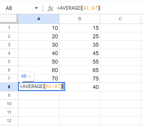
The result in cell A8 would be 40, which is the average of the numbers 10, 20, 30, 40 and 50.

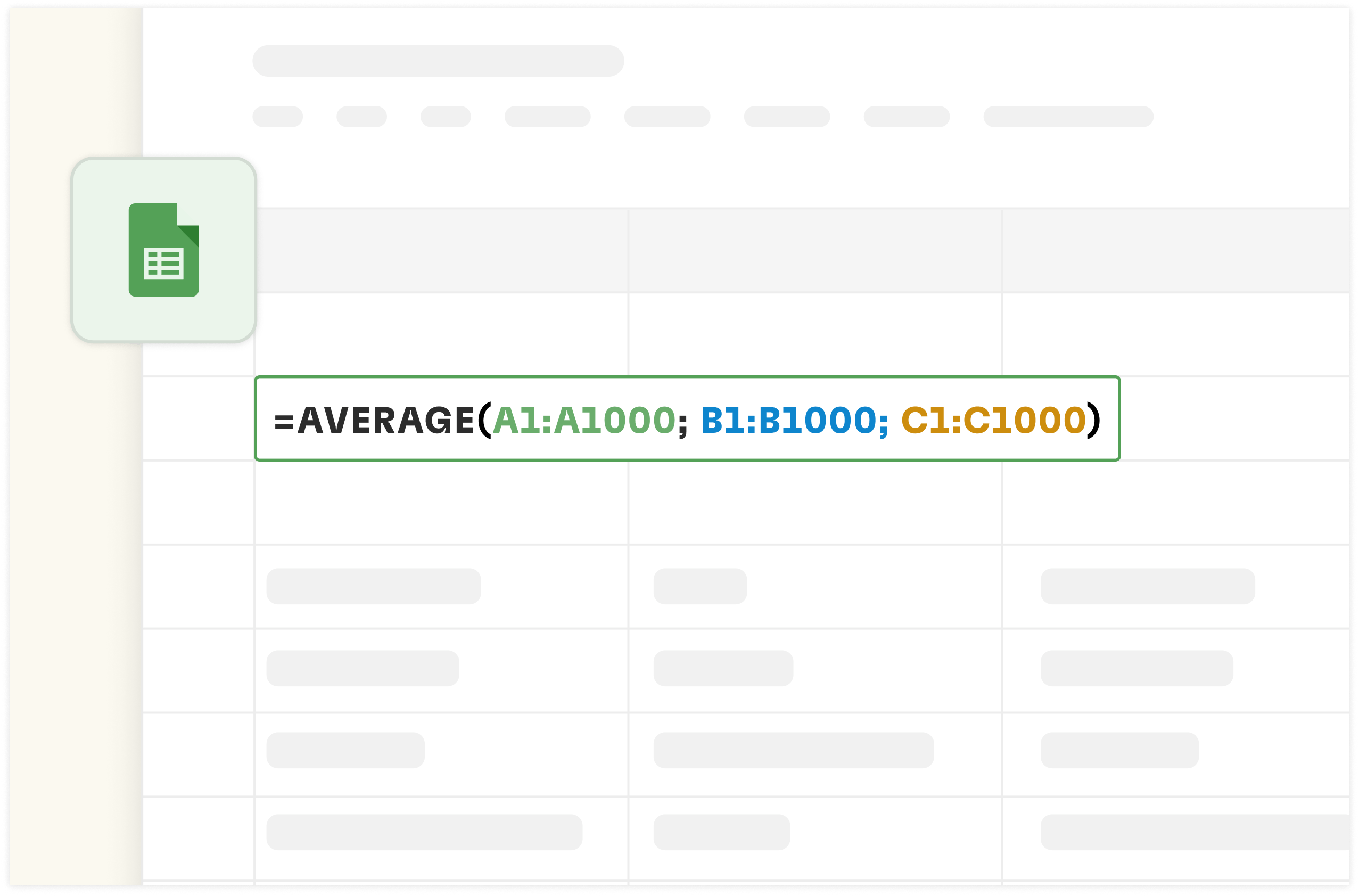
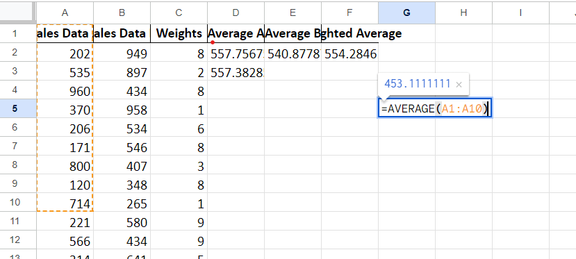
Example 2: Averaging a large dataset

Suppose you have a large dataset of sales numbers in the range A1 through A1000. To calculate the average of this range:

1. Select the cell where you want the average displayed (e.g., cell C2).

2. Type the formula =AVERAGE(A1:A1000)

3. Press Enter.

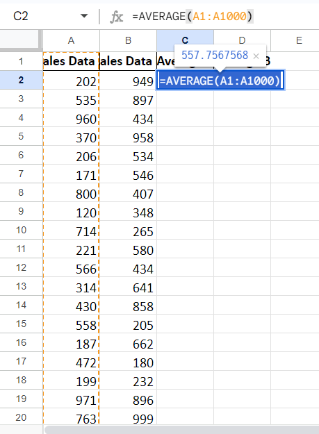
The AVERAGE function will calculate the average of all 1,000 sales numbers and display the result in cell C2.

Tips and Considerations:

• The AVERAGE function can handle numerical and text data but will only include the numerical values in the calculation.

•  If there are any empty cells or non-numerical values in the range, the AVERAGE function will exclude them from the calculation.

• You can also use the AVERAGE function with individual cell references instead of a range, like =AVERAGE(A1, A2, A3).

• The AVERAGE function is commonly used in spreadsheets to summarize and analyze numerical data quickly.

Handling Blank and Text Cells

The standard AVERAGE() function in Google Sheets behaves the same way whether you have blank cells or text cells in the range:

1. Blank Cells: The AVERAGE() function will ignore blank cells and only calculate the average of the numeric values.

2. Text Cells: The AVERAGE() function will also ignore any cells containing text and only calculate the average of the numeric values.

If you want to treat blank cells as zeros when calculating the average, use the standard `AVERAGE()` function and replace the blank cells with zeros before applying the formula. Here's an example:

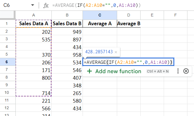
=AVERAGE(IF(A1:A10="",0, A1:A10))

This formula first checks each cell in the range A1:A10 and replaces any blank cells with a zero, then calculates the average of the resulting values.

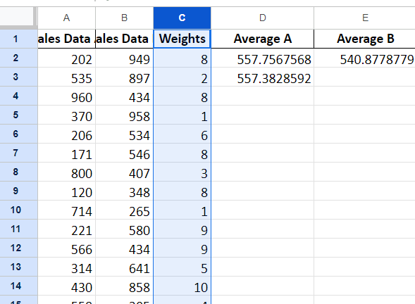
Calculating Weighted Averages

In some cases, you may need to calculate a weighted average, where certain values in the range have a greater influence (i.e. weight) on the final result.

Here is an example of how you can do this in Google Sheets.

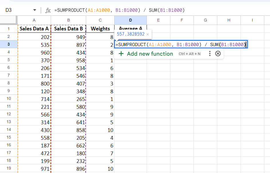
In this example, 

=SUMPRODUCT(A1:A1000, B1:B1000) / SUM(B1:B1000)

Advanced Average Formulas in Google Sheets

AVERAGEIF and AVERAGEIFS Functions

The AVERAGEIF() and AVERAGEIFS() functions allow you to calculate the average of a range based on specific criteria. This is useful when you need to find the average of a subset of your data.

The AVERAGEIF() function takes the following arguments:

=AVERAGEIF(range, criteria, [average_range])

• range: The range of cells to evaluate based on the criteria.

• criteria: The condition that the cells in the range must meet.

• [average_range] (optional): The range of cells to average. If omitted, the function will use the same range as the first argument. 

Example

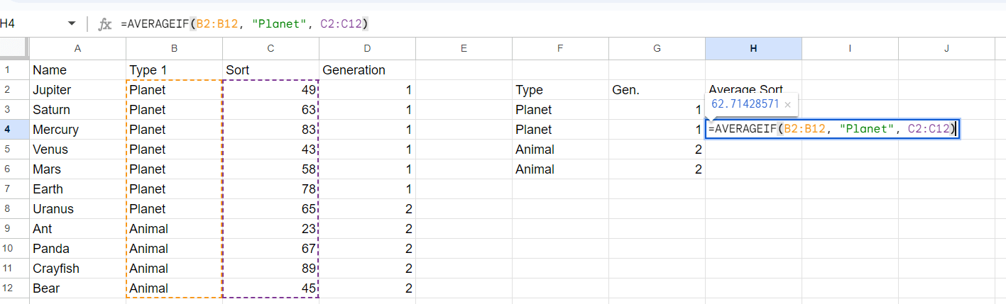
Let’s assume you want to calculate the average of the "Sort" column (Column C) for all items in the "Type" column (Column B) that are labeled as "Planet."

Here’s how the formula would look:

=AVERAGEIF(B2:B12, "Planet", C2:C12)

This formula checks the range B2:B12 for the criteria "Planet" and then averages the corresponding values in the range C2:C12

If you want to input this formula, follow the steps below:

1. Select the cell you want the output to be. In this example, we are using H4

2. Enter the formula =AVERAGEIF(B2:B12, "Planet", C2:C12) and press Enter.

This will calculate the average for all rows where the Type is "Planet" based on their Sort values. Adjust the ranges as necessary if your data range is different.

The AVERAGEIFS function

The AVERAGEIFS function is similar, but allows you to specify multiple criteria:

The AVERAGEIFS function takes the following arguments:

The "range" parameter specifies the cells to evaluate based on the criteria. 

The "criteria" parameter defines the condition that the cells must meet. 

The optional "average_range" parameter allows you to specify a different range for the function to calculate the average.

The criteria can check for conditions like whether a number is greater than, less than, or equal to a certain value.

Formula:

=AVERAGEIFS(average_range, criteria_range1, criteria1, [criteria_range2, criteria2], ...)

In this case, the function will calculate the average of the "average_range" based on all the specified criteria. 

The criteria_range1, criteria_range2, etc. define the ranges where the respective criteria1, criteria2, etc. will be checked.

Overall, these functions provide a flexible way to compute averages for specific subsets of your data.

Example

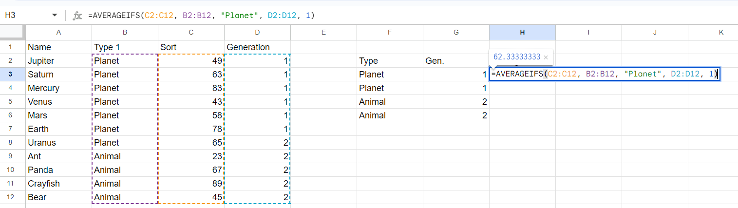
In this example, if you want to calculate the average `Sort` value for rows where the `Type 1` column (Column B) is "Planet" and `Generation` (Column D) is 1, the formula should look like this:

=AVERAGEIFS(C2:C12, B2:B12, "Planet", D2:D12, 1)

Explanation:

C2:C12 is the range where the average is calculated.

B2:B12 is the criteria range to match "Planet".

"Planet" is the criteria for the `Type 1` column.

D2:D12 is the criteria range for `Generation`.

`1` is the criteria for the `Generation` column.

Visualizing Averages with Charts

Google Sheets makes it easy to visualize your average data using various chart types. Once you have calculated your averages, you can create charts such as line charts, bar charts, or scatter plots to display the data more intuitively and visually appealingly.

To create a chart in Google Sheets:

1. Select the range of cells containing your average data.

2. Click the "Insert" menu and select "chart".

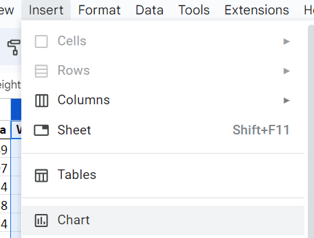
3. Customize the chart settings to suit your needs.

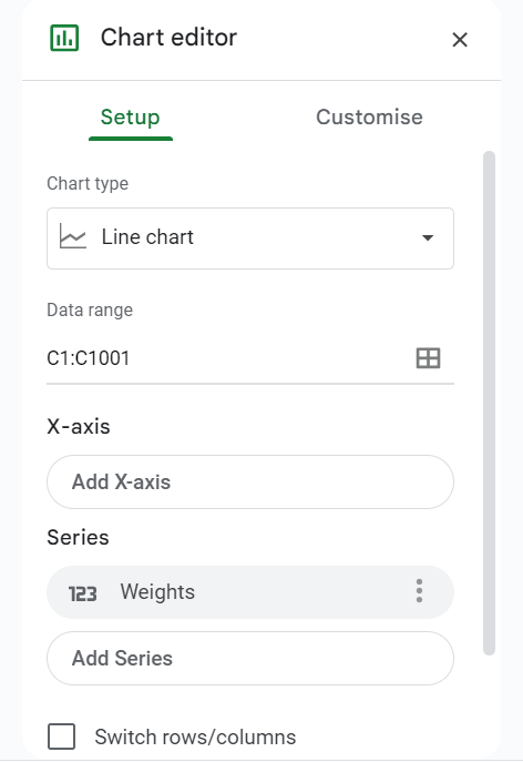
Visualizing your average data can help you easily identify trends, patterns, and outliers, leading to more informed decision-making.

Common Mistakes to Avoid When Using the Google Sheets Average Formula

Avoiding common mistakes when using the Google Sheets average formula will ensure accurate results and save time troubleshooting. 

Look out for some of the most common errors: 

1. Incorrect Cell References: Double-check that you are referencing the correct range of cells in your average formula. Mixing up row and column references or forgetting to include all the desired cells can lead to inaccurate averages.

2. Empty Cells: If there are empty cells within the range you're averaging, the formula will exclude them, skewing the final result. Make sure to remove any blank entries or replace them with zeros if appropriate.

3. Text in Numerical Ranges: The average formula expects a range of numerical values. If there is any text or non-numeric data within the selected cells, the formula will not work correctly. Review your data thoroughly to remove or convert non numerical entries to numbers.

4. Inconsistent Data Types: Similarly, be mindful of mixing data types, such as combining numbers, dates, and text. The average function can only properly calculate numeric values, so any inconsistencies will cause errors.

Here’re some of the best ways to avoid mistakes when using Google Sheets Average formula:

• Prepare Your Data: Before applying the average formula, ensure your data is clean, consistent, and free of any empty or text-based cells.

• Double-Check Cell References: Carefully review the cell range you've specified in the formula to confirm it matches the intended data set.

• Use Descriptive Column/Row Labels: Giving clear names to your data ranges can help you easily identify the correct cells to include in the average calculation.

• Validate Results: After applying the average formula, cross-check the output against your original data to verify the accuracy of the calculation.

How to use AVERAGE in Rows [Easier Alternative]

Rows is your new AI Data Analyst. It combines the backbone of a spreadsheet with the power of ChatGPT to to give business people full autonomy over their data. Just ask in plain language and Rows will handle the rest, whether that's spreadsheet operations, data import or transformations, or running Python code to do code-level analyses.

It’s the new way teams at HP, AWS or Taxfix work with numbers and share their results.

How to use the AVERAGE Function in Rows

You can use the same method and syntax on sheets to calculate averages in Rows.

The most basic way to calculate an average in Rows is to use the AVERAGE() function. This function takes a range of cells as an argument and returns the arithmetic mean of the values in that range.

Syntax

=AVERAGE(followed by the range of cells you want to average, separated by commas). 

For example: =AVERAGE(A1:A10)

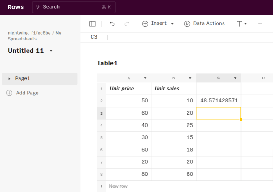
Step 1: Type in the syntax on a separate cell to calculate the average of a specific range in your spreadsheet.

For this example, I calculated the average of the column tagged “unit price”.

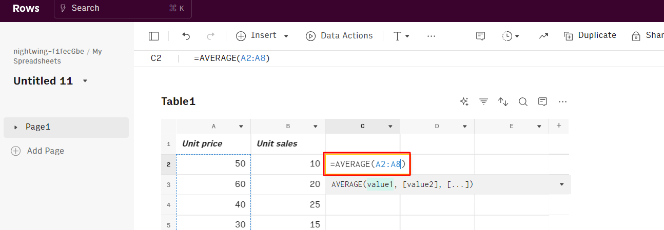
Once you type the syntax, click the “enter tab” on your keyboard and you'll see the average of the data range.

How to use the AVERAGEIF Function in Rows

Returns the average of values in a range if they meet a criterion specified in another range.

Syntax

=AVERAGEIF(range, criterion, [average_range])

• range

Range of values to check against the criterion. Must be of the same size (rows and columns) as average_range.

• criterion

Pattern or test to apply to the range.

• [optional] average_range

Range of values to be averaged.

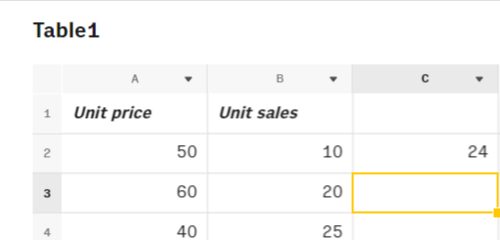
Step 1. Insert the syntax for AVERAGEIF. Ensure you put the specific criterion in quotes.

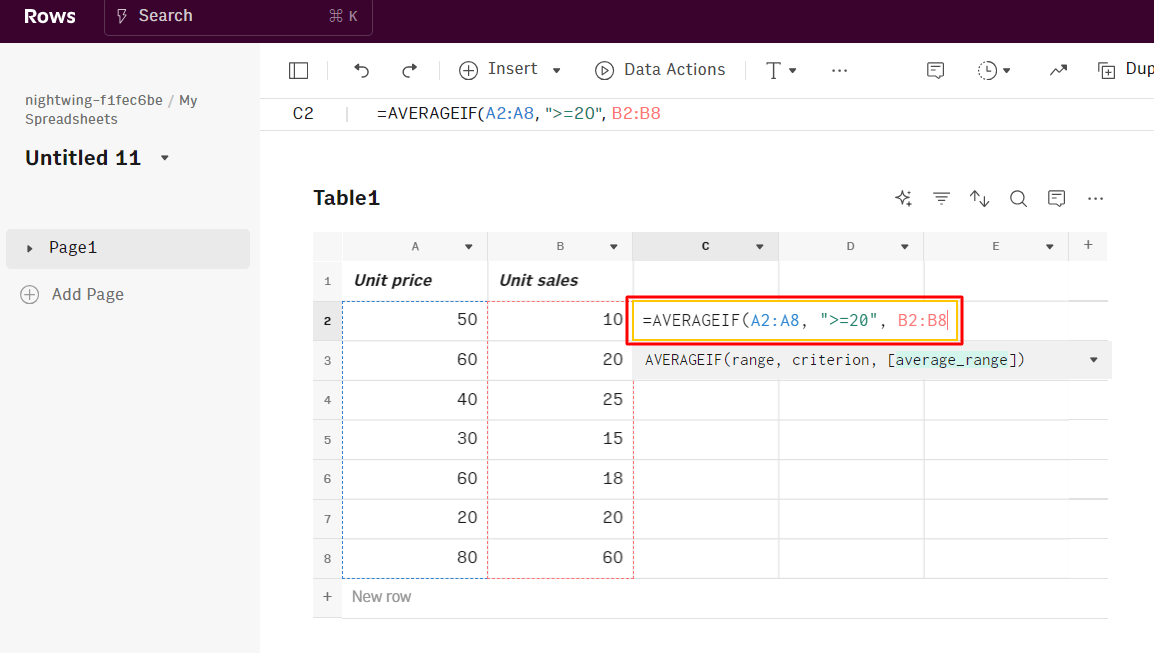
The syntax prompts to get an average of numbers greater than or equal to 20. And the result shows an average of 24.

Why Rows?

In the previous paragraphs, we described how to use the standard AVERAGE functions in Rows. What we haven't described yet is what sets Rows apart from other legacy platform: its AI-first approach to the entire data workflows, from data ingestion, to transformation, and analysis.

Let's dive in:

Feature 1. AI copilot

Rows AI Analyst turns your spreadsheet into something closer to a data science environment. You describe what you want in plain language, and it handles the execution, whether that's spreadsheet operations, data transformations, or running Python code to do the heavy lifting.

It works across four key capabilities:

Spreadsheet-native operations: Standard spreadsheet tasks—pivots, conditional formatting, new columns, charts—happen through conversation instead of clicking through menus or writing formulas.

Example prompts:

→ "Build a pie chart showing share of profit by product" → "Add conditional formatting rule to column D: red if <100, yellow if <150 and green if >150"

Data Ingestion: Pull data directly from PDFs, images, or connected tools without manual copying and pasting.

Example prompts

→ "Import all transactions from my N26 account and classify them as: marketing, software, travel, other" → "Pull keyword data from the last 90 days from Google Search Console"

Multi-step plans: String together multiple dependent steps—build a dashboard, create a calculator from scratch, or execute a series of operations where each step builds on the last.

Example prompts:

→ "Add a column classifying keyword position into brackets: [1-3], [4-10], [10+], then create a pivot showing average CTR by bracket" → "Build a simple dashboard showing the performance of sales people in the last quarter"

Code-level analysis: When you need statistical analysis, machine learning, or custom visualizations that go beyond standard charts, the AI Analyst can write and execute Python code to get there.

Example prompts:

→ "How does my revenue change if my margin increases by 5%?" (what-if analysis) → "How many orders do I need to hit $100k, $500k, and $1M in revenue?" (goal-seek) → "Calculate correlation between keyword position and clicks, then show statistical significance" → "Run a k-means clustering model to segment customers by purchase behavior and visualize the clusters" → "Create a Sankey diagram showing traffic flow from source → landing page → conversion"

See a side-by-side comparison of a price sensitivity analysis in Rows vs. Google Sheets:

Instead of switching between tools or learning specialized syntax, you describe the analysis you want and the AI Analyst figures out how to execute it: it scans your dataset, understands the key variables, and provides what you need.

To access AI in Rows you can either

• click on the ✨ icon, at the bottom right corner of your viewport: this will open a chat UI panel that will work across your spreadsheet. You can ask questions in two modes, Build or Chat, based on whether you want to actually creating elements or just have in-line answers.

• use the ✨ icon at the top right corner of each element: a contextual menu with a few shortcut will open right away allowing you to perform quick actions like summarizing the content or beautify a table

Feature 2. Data Integrations

Rows gives you 50+ data integrations that you can leverage to import and export live data seamlessly into/from the spreadsheet and set up automated data refresh. 

Unlike Google Sheets, this requires no plugin; it’s a built-in native feature, and can be used also with plain language, as mentioned above.

Example of prompts:

• SEO data: "Pull page data from the last 30 days from Google Search Console, including only pages that contain /blog/"

• Finance data: "Pull all transactions from my HSBC account and classify them into: software, marketing, travel expenses, revenue"

• Marketing data: "Use GA4 data to rank the top sources of traffic from mobile in Brazil in the last 30 days"

Curious how Rows can do this? It handles JSONs in the grid and converts them into table format.

Here is another example of how to pull GA4 data via AI in Rows:

And whenever the tool you want to retrieve data from is not in their catalog, Rows gets you covered. Thanks to the custom HTTP source, you can send GET, POST, PUT, and PATCH requests to any endpoint using basic or API token authentication methods.

You feel ready to try it yourself?

💡 Try to make a GET request yourself with our HTTP Request Tester: input the endpoint, the headers and params and visualize the content of the response in a cell.

Or watch the demo below:

Looking for an head start to test Rows integrations? Have a look to our gallery of templates, including our recent Google Analytics reports and OpenAI testers.

Feature 3. PDF/Image extraction

As mentioned above, Rows can ingest data directly from documents and images—not just as static imports, but as structured, editable tables.

• It works with PDFs and multiple image formats (JPEG, PNG, HEIC...)

• You can process batches at once rather than uploading files one by one.

• All extracted data can get merged into a single table you can immediately work with, stay on separate tables or get appended to an existing one.

• You can also add custom extraction instructions to pull exactly what you need. A very common use case is invoices management. By adding the prompt "Extract date, vendor name, VAT amount, total amount, and description", Rows will scan all documents and return a consolidated table with those specific fields—no manual data entry, no error, or formatting issues

Instructions can be enhanced automatically and saved for later. Watch the demo below:

Feature 4. A delightful layout

Rows layout lets you build elegant dashboards that are great to share. See an example of our investor dashboard (numbers are dummy).

Plus, you can embed tables and charts on a website, wiki, or other internal tools with ease.

It’s a simple 4 step process:

1. Choose Embed in the settings menu located in the right-hand corner of the element you want to embed.

2. Click the Share Privately toggle.

3. Click <> Copy code. You can use the Copy link to paste directly into tools that automatically embed via the link - e.g., Notion.

4. Paste the embed code on your website, wiki, or destination tool.

Learn how to use Embed in all the most recent documentation tools, like Notion, Confluence, and Slite.

Fan of Notion? Discover other embed use cases: how to create a chart in Notion and how to import a spreadsheet in Notion.

Your new AI Data Analyst

Extract from PDFs, import your business data, and analyze it using plain language.

Try Rows (no signup)

Supercharge your sheets with Rows

With Rows, you get access to 50+ built-in data source integrations in various domains. 

This makes it easy to ingest data into your table quickly and reduces your team's stress. 

With Rows, you can gather data from various sources in your system. This allows for more detailed analyses and helps your team uncover insights they might miss.

Ready to get started with Rows.com? Start using the product right away for free.