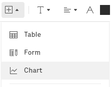
You find the charts option in the Insert
 menu.
menu.

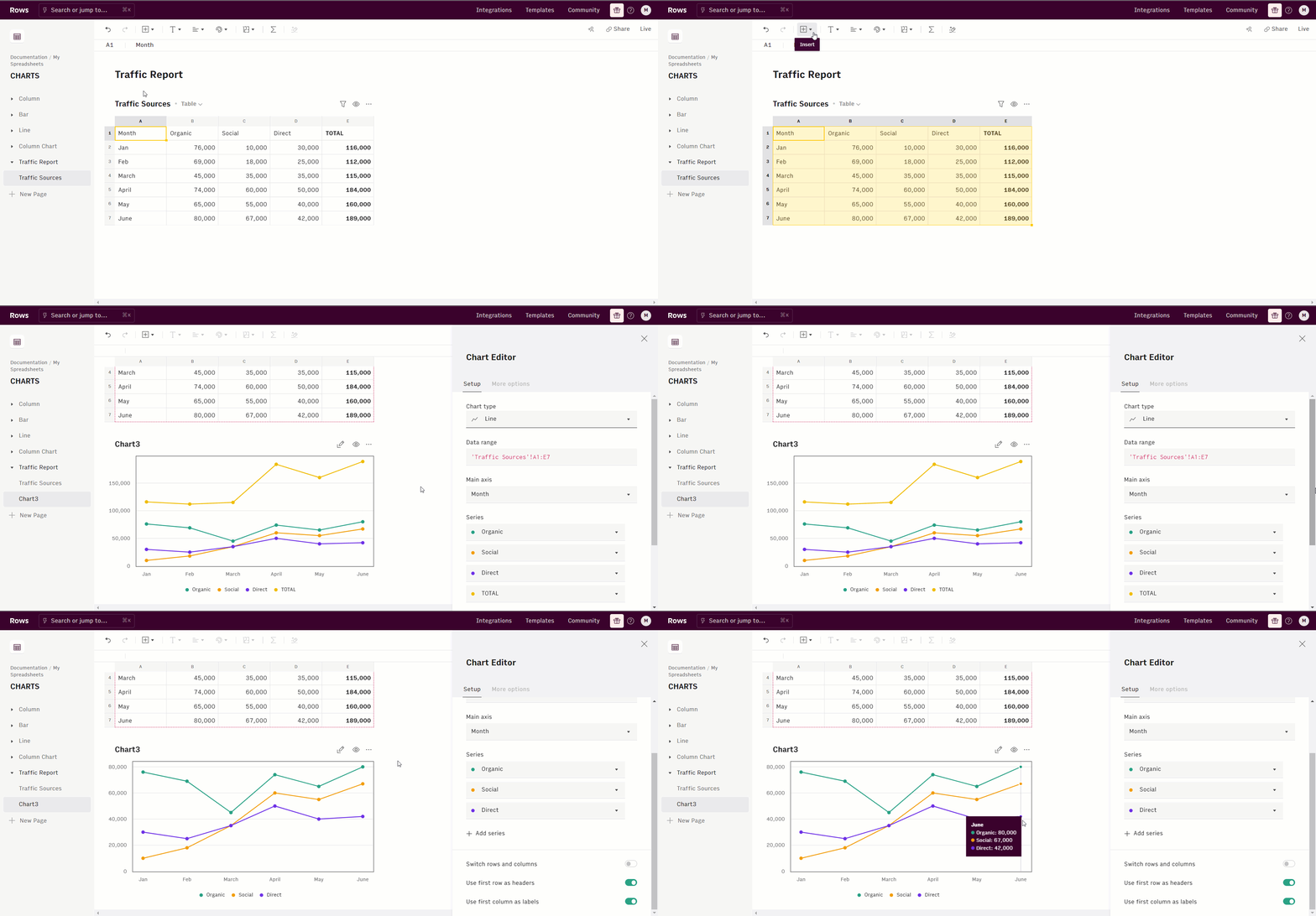
To insert a chart, follow these steps:
- On your computer, open a spreadsheet in Rows.
- Select the cells you want to include in your chart.
- Click Insert > Chart

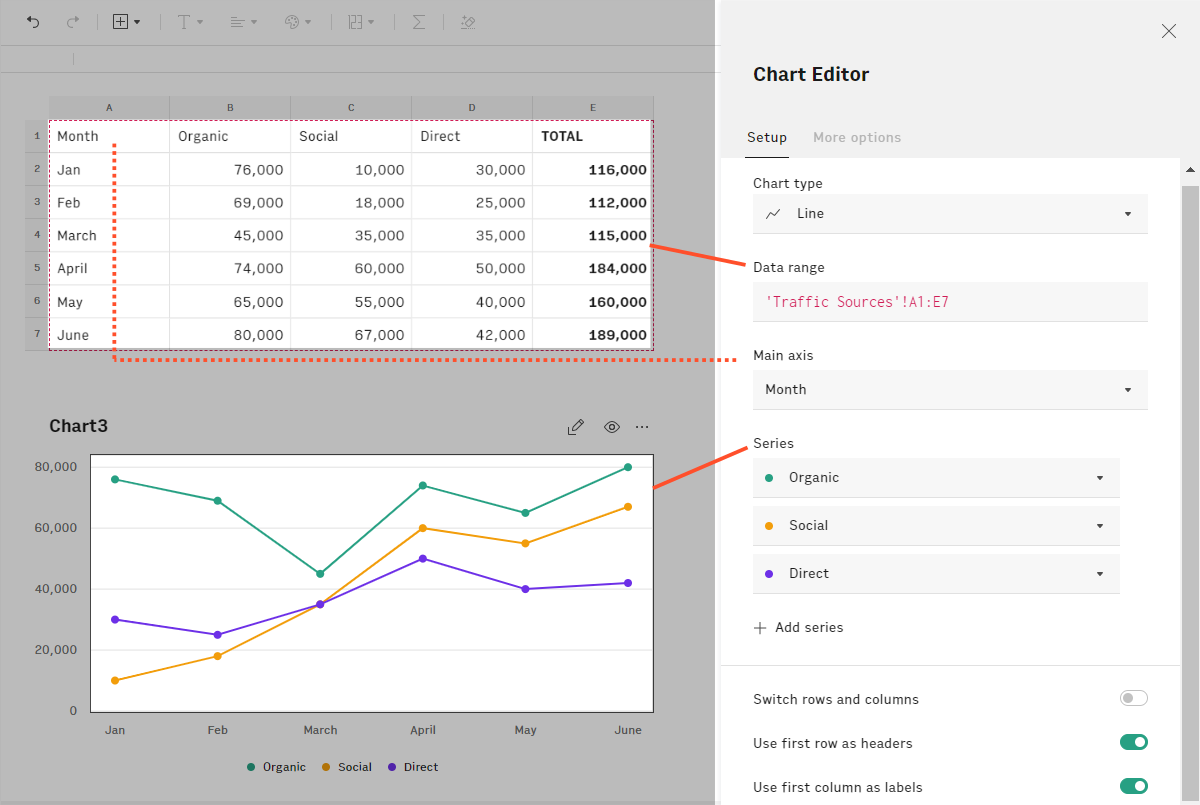
- Configure the chart options in the Chart Editor.

| Field Name | Use To |
|---|---|
| Chart type | Select one of the available chart types. |
| Data range | Define the cell range that stores your chart's data. |
| Main axis | Define the column that stores the data for the main axis. For time-series data, this usually a date column. |
| Series | Update the data series represented in the chart and add or remove specifc series. For example, in a previous illustration, we demonstrated how to remove the "total" series because it distorted the scale of the vertical axis. |
| Switch rows and columns | Switch this toggle to look for series labels in the first column rather than the first row. For example, in the above illustration, this option would be useful if traffic source names were the first colum (A1:A7) rather than the first row (A1:E1) |
Edit your chart
You can change the data range, chart type, and axis settings in the chart editor. You can also rename your chart, delete it, or change its visibility settings in the chart toolbar.

The chart toolbar is visible when you hover your mouse over the chart.
To change the data range, chart type, and axis settings, follow these steps:
- Open a spreadsheet in Rows and locate your chart.
- To change the data range or edit the chart type the series, click the Edit button or open the edit menu and click Edit chart.
- Update the relevant settings in the chart editor.
To change a chart’s visibility:
- Click the Visibility icon. When the Visibility is set to hidden, the chart won’t be visible in live mode.
Anyone who opens the spreadsheet with the live link will no longer see the chart.
To rename a chart:
Double-click the name of the chart and enter the new name.
OR
Open the chart’s Edit
 menu and click Rename.